Model of a generic DC load. The load can be either constant or
variable depending on the value of the parameter mode.
See the model Buildings.Electrical.Interfaces.Load
for more information.
The model computes the current drawn from the load as
P = V i,
where P is the power, V is the voltage and
i is the current.
If the component consumes power, then P < 0. If it feeds
power into the electrical grid, then P > 0.
Consider the simple DC circuit shown in the figure below
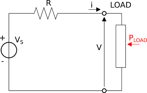
where VS is a constant voltage source, and R is the line resistance. The load has a voltage V across its electrical pins and a current i is flowing through it. If the power consumption drawn by the load is prescribed by the variable PLOAD, the equation that describes the circuit is
VS - R i - PLOAD/i = 0
The unknown variable i appears in a nonlinear equation. This means that in order to compute the current that is drawn by the load, a nonlinear equation has to be solved. If the number of loads increases (as typically happens in real case examples) the number of nonlinear equations to be solved increases too, and the resulting system of nonlinear equations can slow down the simulation. It is possible to avoid such a problem by introducing a linearized model.
The first step to linearize the load model is to define its
nominal voltage conditions Vnom, around which the
equations will be linearized.
The constitutive equation of the load can be linearized around the
nominal voltage condition Vnom as
i = PLOAD/V = PLOAD/Vnom + (V - Vnom)[∂ (PLOAD/V)/ ∂V ]V = Vnom + ₒ((V - Vnom)2),
which leads to the linearized formulation
i ≃ PLOAD (2/Vnom - V/Vnom2).
The linearized formulation approximates the load power consumption (or production), with the approximation error being proportional to (V - Vnom)2. A further approximation has been introduced to improve the approximation of the linearized model even if the voltage is far from the nominal condition. This piecewise linearized approximation instead of approximating the model just in the neighborhood of the nominal voltage Vnom introduces two new points where the model is approximated. The points are at 0.8 Vnom and 1.2 Vnom.
| Equation | Condition |
|---|---|
| i ≃ PLOAD (2/(0.8 Vnom) - V/(0.8 Vnom2)) | V < 8/9⋅ Vnom |
| i ≃ PLOAD (2/(1.2 Vnom) - V/(1.2 Vnom2)) | V ≥ 12/11⋅ Vnom |
| i ≃ PLOAD (2/Vnom - V/Vnom2) | Otherwise |
initMode that can be used to select the
assumption to be used during initialization phase by the homotopy
operator.