The Buildings.Electrical package extends the capabilities of the Buildings library with models for electrical systems, allowing to study building-to-grid integration such as the effect of large scale PV on the voltage of the electrical distribution grid. The package contains models for different types of sources, loads, storage equipment, and transmission lines for electric power. The package contains models that can be used to represent DC, AC one-phase, and AC three-phase balanced and unbalanced systems. The models can be used to scale from the building level up to the distribution level. The models have been successfully validated against the IEEE four nodes test feeder.
The Buildings.Electrical package uses a new type of generalized connector that has been introduced by R. Franke and Wiesman (2014) and is used by the Power Systems Library and the Electric Power Library.
The Modelica Standard Library (MSL) version 3.2.1 has different connectors depending on the type of electric system being modeled. For example, DC and AC continuous time systems have a connector (Modelica.Electrical.Analog.Interfaces.Pin) that differs from the one used by AC models, which use the quasi-stationary assumption ( Modelica.Electrical.QuasiStatic.SinglePhase.Interfaces.Pin).
The generalized electrical connector overcomes this limitation.
It uses a paradigm that is similar to the one used by the
Modelica.Fluid connectors. The generalized connector
is as follows:
connector Terminal "Generalized electric terminal"
extends Buildings.Electrical.Interfaces.BaseTerminal ;
replaceable package PhaseSystem = Buildings.Electrical.PhaseSystems.PartialPhaseSystem "Phase system" ;
PhaseSystem.Voltage v[PhaseSystem.n] "Voltage vector" ;
flow PhaseSystem.Current i[PhaseSystem.n] "Current vector" ;
PhaseSystem.ReferenceAngle theta[PhaseSystem.m] "Optional vector of phase angles" ;
end Terminal;
The connector has a package called PhaseSystem that
contains constants, functions, and equations of the specific
electric domain. This allows to represent different electrical
domains using the same connector, reusing the same standardized
interfaces.
As the electrical connectors of the Modelica Standard Library,
the Terminal has a vector of voltages as effort
variables and a vector of currents as flow variables. The connector
has an additional vector that represents the reference angle
theta[PhaseSystem.m]. If PhaseSystem.m >
0 the connector is overdetermined because the number of
effort variables is higher than the number of flow variables. The
over-determined connectors are defined and used in such a way that
a Modelica tool is able to remove the superfluous but consistent
equations, arriving at a balanced set of equations based on a graph
analysis of the connection structure. The models in the library
uses constructs specified by the Modelica language to handle this
situation Olsson Et Al. (2008).
The connector has a package called PhaseSystem that
allows to represent different electrical domains using the same
connector, reusing the same standardized interfaces. The available
PhaseSystems are contained in the package Buildings.Electrical.PhaseSystems.
Each of the available packages represent a different type of electrical systems. The electrical systems represented are:
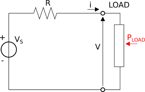
Consider the simple DC circuit shown above, where VS is a constant voltage source and R is a line resistance. The load has a voltage V across its electrical pins and a current i. If the power consumed by the load is PLOAD, the equation that describes the circuit is nonlinear.

If the number of loads increases, as typically happens in grid
simulations, the size of the system of nonlinear equations to be
solved increases too, causing the numerical solver to slow the
simulation. A linearized load model can solve such a problem. All
the load models in the Buildings.Electrical package
have a linearized version. The linearized version of the model can
be selected by setting the boolean flag linearized =
true. Details about the implementation of the linearized
models can be found in Buildings.Electrical.DC.Loads.Conductor
or Buildings.Electrical.AC.OnePhase.Loads.Resistive.
When multiple loads are connected in a grid through cables that
cause voltage drops, the dimension of the system of nonlinear
equations increases linearly with the number of loads. This
nonlinear system of equations introduces challenges during the
initialization, as Newton solvers may diverge if initialized far
from a solution. The initialization problem can be simplified using
the homotopy operator. The homotopy operator uses two different
types of equations to compute the value of a variable: the actual
one and a simplified one. The actual equation is the one used
during the normal operation. During initialization, the simplified
equation is first solved and then slowly replaced with the actual
equation to compute the initial values for the nonlinear systems of
equations. The load model uses the homotopy operator, with the
linearized model being used as the simplified equation. This
numerical expedient has proven useful when simulating models with
more than ten connected loads. All the load models of the Buildings.Electrical package
use the the homotopy operator during the initialization. The
parameter initMode is used to select which simplified
equation should be used by the homotopy operator:
Buildings.Electrical.Types.InitMode.zeroCurrentBuildings.Electrical.Types.InitMode.linearizedMost components have a parameters for the nominal operating
conditions. These parameters have names that end in
_nominal and they should be set to the values that the
component typically have if they are run at design conditions.
Depending on the model, these parameters are used differently, and
the respective model documentation or code should be consulted for
details. However, the table below shows the typical use of the
parameters in various models to help the user understand how they
are used.
| Parameter | Model | Functionality |
|---|---|---|
| V_nominal P_nominal |
Load models | V_nominal is the RMS (Root Mean Square) voltage at
which the load consumes the nominal real power (measured in [W])
P_nominal. When the load model are linearized, the
linearization is done for V = V_nominal. |
| V_nominal P_nominal |
Transmission line models | V_nominal is the RMS (Root Mean Square) voltage at
which the line operates while P_nominal is the power
flowing through it. These values are used in some cases to
automatically select the right cable properties. |
| V_nominal | Storage PVs Wind turbine |
V_nominal is the RMS (Root Mean Square) voltage at
which these components typically operate. Since these model contain
load models, V_nominal can be used for linearization
purposes. |
| V_nominal | Sensors | V_nominal is the RMS (Root Mean Square) voltage of
the system that is currently measured, it can be used to measure
quantities in per unit [pu]. |
Other information about the models and the packages can be found in the info section of each model or sub-packages.
The paper titled A Modelica package for building-to-electrical grid integration won the best paper award at the BauSIM 2014 conference.
Marco
Bonvini, Michael Wetter, and Thierry Stephane Nouidui.
A Modelica package for building-to-electrical grid
integration
BauSIM 2014 Conference, Aachen, Germany, September
2014.
Rudiger
Franke and Hansjorg Wiesmann.
Flexible modeling of electrical power systems - the Modelica
PowerSystems library.
Proc. of the 10th Modelica Conference, Lund, Sweden, March
2014.
Hans Olsson, Martin
Otter, Sven Erik Mattson and Hilding Elmqvist.
Balanced Models in Modelica 3.0 for Increased Model
Quality.
Proc. of the 7th Modelica Conference, Bielefeld, Germany, March
2008.