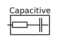
modelCapacitive

Extends from Buildings.Electrical.Interfaces.CapacitiveLoad (Partial model of a capacitive load).
Information
Model of an capacitive load. It may be used to model a bank of capacitors.
The model computes the complex power vector as
S = P + jQ = V ⋅ i*
where V is the voltage phasor and i* is the complex conjugate of the current phasor. The voltage and current phasors are shifted by an angle φ.
The load model takes as input the power consumed by the inductive load and
the power factor pf=cos(φ). The power
can be either fixed using the parameter P_nominal, or
it is possible to specify a variable power using the inputs y or
Pow.
The power factor can be either specified by the parameter pf
or using the input variable pf_in.
The different modes can be selected with the parameter
mode and use_pf_in, see
Buildings.Electrical.Interfaces.Load and
Buildings.Electrical.Interfaces.CapacitiveLoad for more information.
Given the active power P and the power factor pf the complex power Q is computed as
Q = - P tan(arccos(pf)).
The equations of the model can be rewritten as
i1 = (P V1 + Q V2)/(V12 + V22),
i2 = (P V2 - Q V1)/(V12 + V22),
where i1, i2, V1, and V2 are the real and imaginary parts of the current and voltage phasors.
The nonlinearity of the model is due to the fact that the load consumes the power specified by the variables P and Q irrespectively of the voltage of the load.
When multiple loads are connected in a grid through cables that cause voltage drops, the dimension of the system of nonlinear equations increases linearly with the number of loads. This nonlinear system of equations introduces challenges during the initialization, as Newton solvers may diverge if initialized far from a solution, as well during the simulation. In this situation, the model can be parameterized to use a linear approximation as discussed in the next section.
Linearized model
Given the constraints and the two-dimensional nature of the problem, it is difficult to find a linearized version of the AC load model. A solution could be to divide the voltage domain into sectors, and for each sector compute the best linear approximation. However the selection of the proper approximation depending on the value of the voltage can generate events that increase the simulation time. For these reasons, the linearized model assumes a voltage that is equal to the nominal value
i1 = (P V1 + Q V2)/VRMS2,
i2 = (P V2 - Q V1)/VRMS2,
where VRMS is the Root Mean Square voltage os the AC system. Even though this linearized version of the load model introduces an approximation error in the current, it satisfies the constraints related to the ratio of the active and reactive powers.
Initialization
The initialization problem can be simplified using the homotopy operator. The homotopy operator uses two different types of equations to compute the value of a variable: the actual one and a simplified one. The actual equation is the one used during the normal operation. During initialization, the simplified equation is first solved and then slowly replaced with the actual equation to compute the initial values for the nonlinear systems of equations. The load model uses the homotopy operator, with the linearized model being used as the simplified equation. This numerical expedient has proven useful when simulating models with more than ten connected loads.
The load model has a parameter initMode that can be used to select
the assumption to use during the initialization phase by the homotopy operator.
The choices are between a null current or the linearized model.
Parameters
| Type | Name | Default | Description |
|---|---|---|---|
| Modeling assumption | |||
| Boolean | linearized (from Load) | false | If true, the load model is linearized |
| Buildings.Electrical.Types.Load | mode (from Load) | Buildings.Electrical.Types.Load.FixedZ_steady_state | Type of load model (e.g., steady state, dynamic, prescribed power consumption, etc.) |
| Boolean | use_pf_in (from CapacitiveLoad) | false | If true, the power factor is defined by an input |
| Nominal conditions | |||
| Modelica.Units.SI.Power | P_nominal (from Load) | 0 | Nominal power (negative if consumed, positive if generated). Used if mode <> Buildings.Electrical.Types.Load.VariableZ_P_input |
| Modelica.Units.SI.Voltage | V_nominal (from Load) | Nominal voltage (V_nominal >= 0) | |
| Real | pf (from CapacitiveLoad) | 0.8 | Power factor |
| Initialization | |||
| Buildings.Electrical.Types.InitMode | initMode (from Load) | Buildings.Electrical.Types.InitMode.linearized | Initialization mode for homotopy operator |
Connectors
| Type | Name | Default | Description |
|---|---|---|---|
| Modelica.Blocks.Interfaces.RealInput | y (from Load) | Fraction of the nominal power consumed | |
| Modelica.Blocks.Interfaces.RealInput | Pow (from Load) | Power consumed | |
| Buildings.Electrical.Interfaces.Terminal | terminal (from Load) | Generalized electric terminal | |
| Modelica.Blocks.Interfaces.RealInput | pf_in (from CapacitiveLoad) | Power factor |
Components
| Type | Name | Default | Description |
|---|---|---|---|
| Modelica.Units.SI.Voltage[:] | v (from Load) | terminal.v | Voltage vector |
| Modelica.Units.SI.Current[:] | i (from Load) | terminal.i | Current vector |
| Modelica.Units.SI.Power[PhaseSystem.n] | S (from Load) | PhaseSystem.phasePowers_vi(v, -i) | Phase powers |
| Modelica.Units.SI.Power | P (from Load) | Power of the load (negative if consumed, positive if fed into the electrical grid) |
Revisions
-
January 29, 2019, by Michael Wetter:
Addedreplaceablefor terminal. -
May 26, 2016, by Michael Wetter:
Moved function call toPhaseSystem.thetaRefout of derivative operator as this is not yet supported by JModelica. - September 4, 2014, by Michael Wetter:
Revised documentation. - August 5, 2014, by Marco Bonvini:
Revised documentation. -
January 2, 2012, by Michael Wetter:
First implementation.