.BusinessSimulation.Examples.HealTheWorld

Information

This information is part of the Business Simulation Library (BSL). Please support this work and ► donate.

Using the classes in the →CausalLoop package we can quickly start out with a model that captures the important dynamics in a system. This simplified model of world dynamics is given by Hartmut Bossel [25] who reduces the world system to four main variables indicating the state of the world: population, consumption, environmental load, and societal action.

These states or stocks may be initialized with a value of 1.0 representing the respective current level, i.e., an index. In the next step, we must identify direct causal influences between the model variables, i.e., a change in A will affect B (A → B). To more precisely capture the dynamics of the system we may ask ourselves for any impact: If A increases by r_A percent, what will be the fractional rate (r_B) of change for B?. The elasticity coefficient is simply the factor of proportionality between the fractional rates and we can use it to embedd the stocks in a dynamic model of impact as shown in the diagram below.

DiagramView

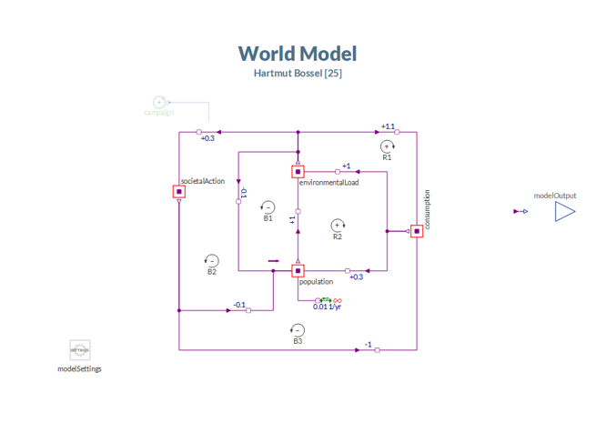For example, we state that a change in the level of the world population will affect a change in the level of environmentalLoad and that the polarity for this relation is positive, i.e., an increase will cause an increase and, conversely, a decrease will cause a decrease. We further assume the percentage change in the level of environmentalLoad to be equivalent to that in the population and accordingly we have set coefficient = +1.0 for the relation (r1) between the two stocks.

The elasticity coefficient for the impact of societalAction upon the level of consumption is set to -1.0, which indicates that any fractional increase in societal action will cause a decrease in consumption at the same fractional rate.

Since all dynamics in a model are solely driven by relative changes, the model is in equilibrium initially, i.e., there will be no dynamics. Two typical questions are of interest in using such a model:

• What will happen if there is some exogenous impact to one or more system states?


• If the system turns out to be instable,i.e., grow or deteriorate without bounds, what can be done?

In this example, we will assume that the population will grow exponentially during the next 10 years at a fractional rate of 1% per year. As a potential intervention, we are considering a public awareness campaign that will start one year into the simulation and last for three years. In the model the intervention (campaign) will affect the elasticity coefficient for the impact of environmentalLoad upon societalAction, which in the base run settings is +0.3. The effect upon the coefficient is modeled as a multiplication; campainTarget = 1/0.3 implies that at the end of the intervention the elasticity coefficient will have risen to a value of +1.0—tightly coupling societalAction to environmentalLoad.

The simulation results for the base run (without intervention) and the policy run (with intervention) are shown in the plots below:

Simulation Plots

Notes

While this, of course, is a toy model, system dynamics modelers coming from other tools may take a moment to reflect upon the following:

• This model fits a single page and has just four stocks—how would this model look in conventional system dynamics tools?


• The causal loop (B1)between population and environment introduces a cycle with regard to variables that are not stocks (e.g., rates of flow to the stocks); the compactness of modeling that we see here is possbile, because Modelica allows algebraic next to differential equations(→DAE).


• Finally, we also see the improved reusability of object-oriented models at work when we consider that we may simply remove the exponential growth process from population and connect it to consumption without having to change anything else in the model.

See also

SoftwareReleaseProject

Contents

Name	Description
Theta	Parameter definitions for the Base Case

Revisions

• Added in v2.0.0.


• Moved check for campaignStart from min attribute to assert statement to guarantee that attribute values are presented in evaluated form (e.g., as structural parameter values); modelSettings.modelStartTime has fixed = false.