This information is part of the Business Simulation Library (BSL). Please support this work and ► donate.
This introductory example continues the example given in the
→Tutorial
(please read that section first, if you have not done so already).
Here we consider a simple production chain for a company (e.g.,
ACME) producing a durable good (e.g., intruder alarm systems).
Products will be produced at a constant rate of 100 units
per month [#/mo]. The finished goods will be collected
in a finished-goods inventory from where they will be
shipped to customers. The inventory will be empty at the start of
the simulation.
In this introductory example we will assume that there are only first-time purchases and that the rate of purchasing is also the rate of shipment to the customers. Initially the purchase rate will be 10 units per month, but due to some marketing initiative we assume that starting in month six the rate will ramp up to 100 units per month within 18 months after which it will remain at that level.
Units will remain in use for an average useful life of 5 years. After the useful life has expired, the units will be discarded. In this example, we will not consider replacement purchases.
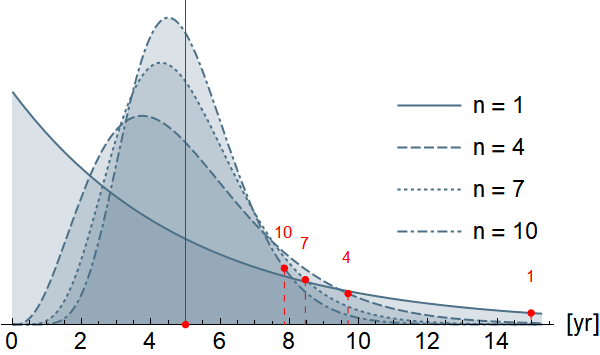
The graph below shows different distributions for the useful
life given an average life of 5 years. The order of the DelayN
component determines the variance for the lifetime distribution.
The dashed red lines show the 95th percentil and the red value
above indicate the corresponding order n. Since we
assume, that 95% of the products will have been discarded after 10
years, it turns out that n = 4 produces a delay
distribution matching the assumption.
 |
In the lower half of the diagram we have included an event-driven process chain (EPC) model typically used in Business Process Modelling (BPM). It offers a nice analogy and allows the transition to a system dynamics perspective coming from that background: While the process is valid for a single unit, in the continuous time simulation we are aggregating the processes (green) and events (red) over time. An event will thus turn into a stock counting the amount of "material" that is in a corresponding state at and given time. A process corresponds to a transition between states at a certain rate given as entities per period.
EPC always start and end with an event and accordingly we always
have to start and end with a stock. In this case the first event is
"hidden" as a stock with an infinite capacity inside the
component of type Growth. AvailableProducts
corresponds to the stock inventory, while "product
received" pertains to installedBase.
A lot of components will refer to variables contained in
modelSettings. There should always be an instance of
that class in the top level scope of any model.
Tutorial.StrategicBusinessSimulation, SimpleProductionChainII, SimpleProductionChainIII, DelayN
| Name | Description |
|---|---|
|
|
Expandable connector for model output |