The default parameters lead to periodic results. Possible
parameter changes to obtain chaotic behavior are noted in the
documentation of the respective subpackage.
Be curios, try different parameter settings to
explore the path from periodic behaviour to chaos - in many cases
you see bifurcation, i.e. different attractors.
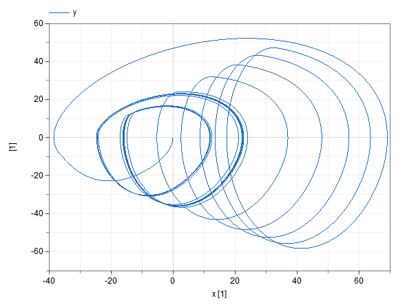
Note that at the beginning a transient process takes place, dependent on the initial conditions. It might be necessary to continue the simulation, as shown for the analytic equations of the ChaoticOscillator proposed by [Tamasevicius2005] :
 |
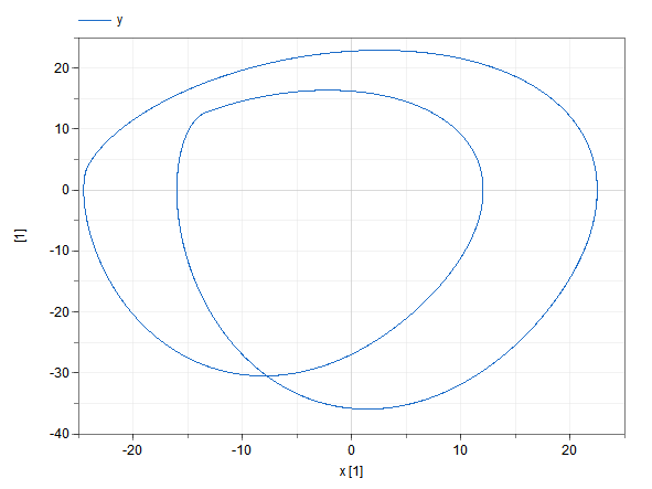 |
| Fig. 1 a=0.75: y vs. x initial transient | Fig. 2 a=0.75: y vs. x after one continuation |
The results meant for plotting are labeled. Normally plot one result variable versus the other, in this example y vs. x and / or z vs. x. Of course the initial transient depends on the initial conditions.
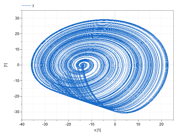
For default parameters, the results converge to a fixpoint. In certain parameter regions only one fixpoint is present. Changing parameters, it might happen that one of two fixpoitns is reached, dependent on the inintial conditions. This is called bifurcation and might happen mutliple times. In the end this leads to chaotic behaviour: Smallest differences in initial conditions lead to dramatically different results. Note that of course the results are strongly dependent on the implementation details of the solver, too.
 |
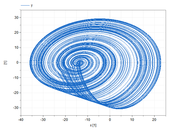 |
| Fig. 3 a=0.35: y vs. x initial transient | Fig. 4 a=0.35: y vs. x after one continuation |
Most circuits (except Lotka-Volterra) are implemented in different flavours:
The main differences between IdealCircuit and ImprovedCircuit are:
| Component | IdealCircuit | ImprovedCircuit |
|---|---|---|
| Diode model | A simple diode according to Shockley equation is used. | A more sophisticated diode model with linear continuation of the characteristic and optional temperature dependency. |
| Operational amplifiers | ideal 3 pin model: input currents are zero, differential input voltage is zero, amplification is infinite, output voltage is not limited | more sophisticated opAmp model: input currents are zero, differential input voltage is zero, amplification is finite, output voltage is limited by suppply voltage |
Slightly different results of the different implementations may
occur, they stem from more detials that are taken into account with
the more sophistiacted implementation.
Note that for the more sophisticated OpAmp-model IdealizedOpAmp3Pin
from this library is used instead of
IdealizedOpAmpLimited from MSL to get rid of the implementation
with smooth (which allows tools to avoid events when
saturating!) and noEvent (which suppresses
events!).
All circuits can be built in reality with simple electronic components. If an inductance is used, its resistance is modeled, too. The ohmic losses of an inductance cannot be neglected.
The equations are summarized in this document.
Note: In the subdirectory Resources.Reference reference results for all examples are stored.