
classUncertaintyInfo
Extends from Modelica.Icons.Information (Icon for general information packages).
Information
This is the information about the quality of a parameter value and, thus, an essential part of a credible model. Besides a mathematical description of the uncertainty (see e.g. [Otter2022]), also the same information as for the traceability of parameter value needs to be given:
- source: origin of the uncertainty determination (e.g. Estimated), see traceability.
- info (optional): a short textual explanation how the uncertainty was determined.
- reference (optional): identifies the resource where the uncertainty determination is described, for example web-address, DOI, ISBN, internal report ID of a document, data-sheet etc. The referenced resource must be stored in a way that avoids accidental manipulation, e.g., in a version control system with a given hash, in order to retain the reference information reliably.
Additionally, the mathematical description of uncertainties of scalars and of arrays/tables must be provided. Particular descriptions provided with the library are collected in package Types.Uncertainty.
The treatment implemented in the library is focused on providing the information in a way that it can be used by models described with the Modelica language, FMI or SSP. Furthermore, not only physical/measured quantities are taken into account, but the same description form is also used to define requirements or specifications. For example, a simulation result must match a reference result with some uncertainty, or the result of a design must match some criteria that is specified with an uncertainty description.
Every physical quantity has inherent limits. Therefore, the upper and lower limits of a scalar value need to be defined, independent of the kind of the mathematical description of the uncertainty. For this reason, the minimum information to be provided for a scalar parameter with an uncertainty description of any kind is:
- nominal – the nominal value of the scalar (e.g., determined by calibration).
- lower – the lowest possible value of the uncertain scalar.
- upper – the highest possible value of the uncertain scalar.
Often, it is inconvenient to provide absolute ranges and instead, relative or absolute deviations are more practical. In the eFMI standard (Section 3.2.4) tolerances for reference results are defined in a similar way as tolerances for numerical integration algorithms. Due to its generality, this description form of eFMI is used here as well:
- nominal – nominal value of the scalar
- relTol – relative tolerance of limits with respect to nominal (default = 0.0).
- absTol – absolute tolerance of limits with respect to nominal (default = 0.0).
The lower and upper values are computed from these parameters in the following way:
tol   = max(absTol, relTol*|nominal|)
lower = nominal − tol
upper = nominal + tol
Example
The resistance of an electrical resistor can be defined using following tolerances:
- 200 Ω ± 5 % – limits defined with relTol = 0.05 (absTol = 0 Ω).
- 200 Ω ± 10 Ω – limits defined with absTol = 10 Ω (relTol = 0).
There is a huge literature on the mathematical description of uncertainties. [Riedmaier2021] provides a comprehensive literature overview. In [Bouskela2011], some constructs are proposed to describe uncertain values in the Modelica language. In the Credibility Library, the following uncertainty descriptions are currently provided for scalar Real parameters, see Types:
| Uncertainty name | Parameters | Uncertainty type |
|---|---|---|
| Interval |
nominal, lower, upper
|
epistemic |
| Uniform |
nominal, lower, upper
|
uniform distribution |
| TruncatedNormal |
nominal, lower, upper, stdDev
|
truncated normal distribution |
| IntervalTolerance |
nominal, relTol=0, absTol=0
|
epistemic |
| UniformTolerance |
nominal, relTol=0, absTol=0
|
uniform distribution |
| TruncatedNormalTolerance |
nominal, relTol=0, absTol=0,
stdDevFactor=3
|
truncated normal distribution |
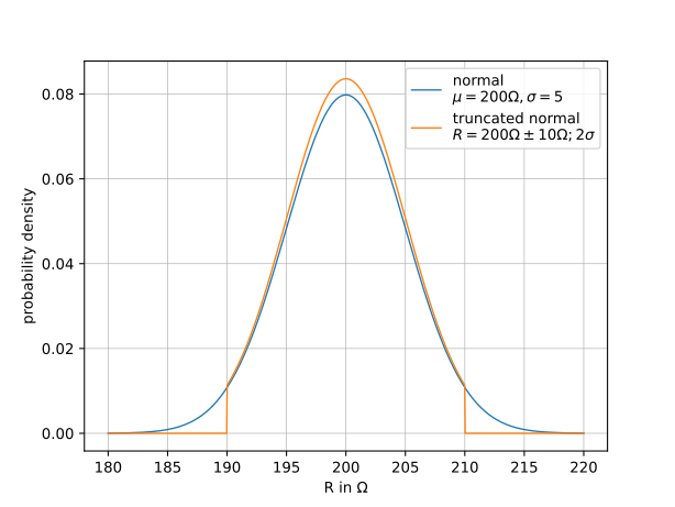
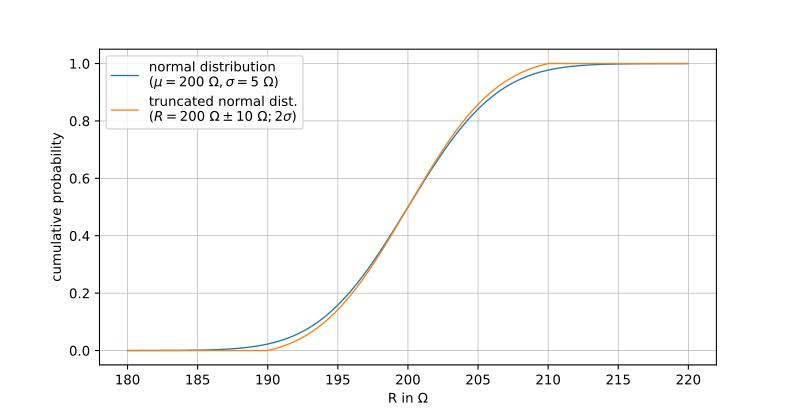
An example for a TruncatedNormalTolerance uncertainty of the abovementioned resistance is given in the next two figures:
Array uncertainty
Arrays occur in system modelling and analysis in various ways:
- Submodels are often approximated by tables of a characteristic property that have been determined by measurements, for example a table defining friction torque as function of relative angular velocity, or a table defining mass flow rate through a valve as function of valve position. Tables of this kind are basically defined with two or more dimensional arrays.
- Inputs of a system are often defined by tables as function of time.
- Outputs of a system might be checked against reference outputs (for example, determined from the previous version of the model or tool, from another tool or from an analytically known solution) defined by tables as function of time. The computed solution is then required to be within uncertainty ranges of the reference tables.
All these examples have parameter arrays, where the uncertainties of the array elements need to be described.
If a characteristic is determined by detailed measurements, then typically for every element upper and lower limits are known from the available measurement data. This means that the measurements can be summarized by a nominal array that has been determined by the calibration process and arrays lower and upper of the same size that define lower and upper limits, so all measured data of the respective characteristics is between these limits. Furthermore, it must be defined how to interpolate between the table values, given the vectors of the independent variables (an n-dimensional table is defined by n vectors of independent variables). Often, linear interpolation is used for tables derived from measurements.
An envisaged uncertainty description with generic parameterization of 2-dim. array can be demonstrated in the following example. The vectors of the two independent variables are u1 = [0.1, 0.2, 0.3, 0.4] and u2 = [10, 20, 30]. The nominal array is a matrix of size [4, 3] and, e.g., of values [110 120 130; 210 220 230; 310 320 330; 410 420 430] (i.e. y = 230 is the nominal value for u1 = 0.2 and u2 = 30). Both the lower and upper limits are matrices of size [4, 3] as well and have exemplary values lower = [11 12 13; 21 22 23; 31 32 33; 41 42 43] and upper = [119 129 139; 219 229 239; 319 329 339; 419 429 439]. Thus, e.g. the uncertain table value of u1 = 0.2 and u2 = 30 (i.e. array element [2, 3]) must be in the range [23 … 239].
Convex scaling by uncertain parameter λ
The question arises how a parameter array can be used to compute the uncertainty distributions of output variables. For scalar parameters, the standard Monte Carlo simulation method is based on the approach to draw sufficient numbers of random numbers according to the respective distributions and for each set of selected parameter values perform a simulation. Such a procedure might not be directly applicable to parameter arrays, because randomly selected elements of an array might give a table that does not represent physics (for example, if the table output is a monotonically increasing function of the input, then this property might be lost if table elements are randomly selected).
For simplicity, the following method is used for 1-dim. tables in the Library. A generalization to multi-dimensional tables is straightforward. A 1-dim. table defines a function y = f (u ) that computes the output y from the input u by interpolation in a table, cf. Modelica.Blocks.Tables.CombiTable1Ds. The table is defined as "table[i,j]" with the first column "table[:,1] = u[:]" which contains the grid points ui, and the second column "table[:,2] = y[:]" which contains the data yi to be interpolated. This "table[i,j]" is computed from the given matrix "uncertainty" by a convex combination utilizing uncertain parameter λ. Hereby, the matrix "uncertainty" contains
- grid values "uncertainty[:,1] = u[:]",
- vector of nominal values "uncertainty[:,2] = nominal[:]",
- vector of lower limits "uncertainty[:,3] = lower[:]" and
- vector of upper limits "uncertainty[:,4] = upper[:]".
The convex combination is defined in a way that λ = −1 results in "y[i] = lower[i]", λ = 0 results in "y[i] = nominal[i]" and λ = 1 results in "y[i] = upper[i]", in particular:
![Equation to calculate y[i] by convex combination utilizing lambda](resources/Credibility/Resources/Images/equationConvexCombination.png)
A realization can be seen in Credibility.Table1D
where "uncertainty" table is in fact defined by parameter uncertainty.table.
In this record, the abovementioned calculation is done in the function
getTableLambdaByInterval.
There is also implemented an alternative calculation of "table[i,j]" called
getTableLambdaByTolerance
utilizing – either relative or absolute –
tolerances.