This package contains models of sensors. There are models with one and with two fluid ports.
When selecting a sensor model, a distinction needs to be made whether the measured quantity depends on the direction of the flow or not, and whether the sensor output signal is the product of the mass flow rate and a medium property.
Output signals that depend on the flow direction and are not multiplied by the mass flow rate are temperature, relative humidity, water vapor concentration X, trace substances C and density. For such quantities, sensors with two fluid ports need to be used. An exception is if the quantity is measured directly in a fluid volume, such as modeled in models of the package IBPSA.Fluid.MixingVolumes. Therefore, to measure for example the outlet temperature of a heat exchanger, the configuration on the left in the figure below should be used, and not the configuration on the right. For an explanation, see Modelica.Fluid.Examples.Explanatory.MeasuringTemperature.
| Correct use | 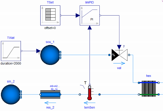 |
|---|---|
| Not recommended | 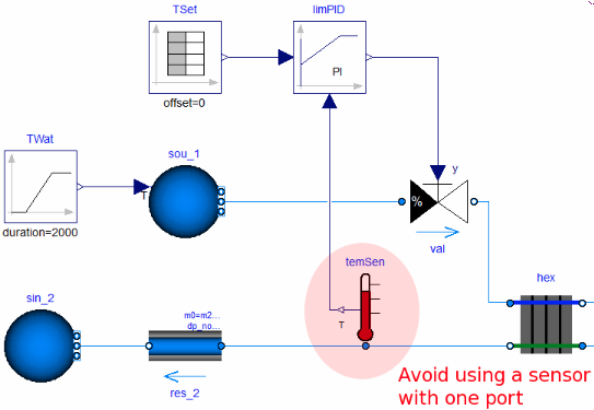 |
Except for the mass flow rate sensor, all sensors with two ports
can be configured as dynamic sensors or as steady-state sensor. For
numerical reasons, if the sensor output signal is not
multiplied by the mass flow rate, then it is strongly suggested to
configure these sensors as a dynamic sensor, which the default
setting. Configuring a sensor as a dynamic sensor is done by
setting the time constant to a non-zero value. Typically, setting
tau=10 seconds yields good results. For
tau=0, numerical problems may occur if mass flow rates
are close to zero.
If the sensor output signal is the product of mass flow rate
times a measured fluid property, such as sensors for volumentric
flow rate or enthalpy flow rate, then the sensor is by default
configured as steady-state sensor. These sensors may be configured
by the user as a dynamic sensor by setting tau > 0,
but there is typically little benefit as these sensors typically do
not cause numerical problems. The reason is that these sensors
multiply the quantity that is carried by the flow, such as specific
enthalpy h by the mass flow rate ṁ to output the
measured signal Ḣ=ṁ h. Hence, as the mass flow rate goes
to zero, the sensor output signal also goes to zero, which seems to
avoid numerical problems.
For static pressure measurements, sensors with one or with two ports can be used for all connection topologies.
The table below summarizes the recommendations for the use of sensors.
| Measured quantity | One port sensor | Two port sensor | |
|---|---|---|---|
steady-state (tau=0) |
dynamic (tau > 0) |
||
| temperature relative humidity mass fraction trace substances specific enthalpy specific entropy |
use only if connected to a volume | avoid | recommended |
| volume flow rate enthalpy flow rate entropy flow rate |
- | recommended | recommended |
| pressure | recommended | recommended | recommended |
If a sensor is configured as a dynamic sensor by setting
tau > 0, then the measured quantity, say the
temperature T, is computed as
τ dT ⁄ dt = |ṁ| ⁄ ṁ0 (θ-T),
where τ is a user-defined time constant of the sensor (a suggested value is around 10 seconds, which is the default setting for the components), dT ⁄ dt is the time derivative of the sensor output signal, |ṁ| is the absolute value of the mass flow rate, ṁ0 is the user-specified nominal value of the mass flow rate and θ is the temperature of the medium inside the sensor. An equivalent physical model of such a sensor would be a perfectly mixed volume with a sensor that outputs the temperature of this volume. In this situation, the size of the volume would be V=τ ṁ0 ⁄ ρ, where ρ is the density of the fluid.
For the sensor IBPSA.Fluid.Sensors.TemperatureTwoPort,
by setting transferHeat = true, heat transfer to a
fixed ambient can be approximated. The heat transfer is computed
as
τHeaTra dT ⁄ dt = (TAmb-T),
where τHeaTra is a fixed time constant and
TAmb is a fixed ambient temperature. Setting
transferHeat = true is useful if the sensor output
T is used to switch the mass flow rate on again. If
transferHeat = false, then the sensor output T
remains constant if the mass flow rate is zero and hence a fan or
pump controller that uses this signal may never switch the device
on again. If the sensor output T is not used to switch on
the mass flow rate, then in general one can use
transferHeat=false.
Note that since in practice the heat transfer is due to a combination of ambient temperature and upstream or downstream fluid temperature, for example by two-way buoyancy-driven flow inside the duct or pipe, the model uses as an approximation a fixed ambient temperature. Since the sensor is not affecting the temperature of the medium, this approximation of the heat transfer does not add or remove heat from the fluid.
For the sensor IBPSA.Fluid.Sensors.TemperatureTwoPort, if both dynamic effects are enabled, then the output T is computed as
dT ⁄ dt = |ṁ| ⁄ ṁ0 (θ-T) ⁄ τ + (TAmb-T) ⁄ τHeaTra.
The above equation is implemented in such a way that it is differentiable in the mass flow rate.
Note that the implementation of the dynamic sensors does not use the model IBPSA.Fluid.MixingVolumes. The reason is that depending on the selected medium model, the mixing volume may introduce states for the pressure, species concentration, trace substance, specific enthalpy and specific entropy. Not all states are typically needed to model the dynamics of a sensor. Moreover, in many building system applications, the sensor dynamics is not of concern, but is rather used here to avoid numerical problems that steady-state models of sensors cause when flow rates are very close to zero.