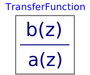
blockTransferFunction
Discrete-time Transfer Function block
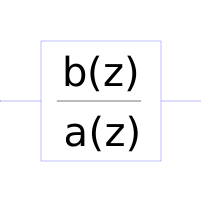
Extends from Clocked.RealSignals.Interfaces.PartialClockedSISO (Block with clocked single input and clocked single output Real signals).
Information
The discrete transfer function block defines the transfer function between the input signal u and the output signal y. The numerator has the order nb-1, the denominator has the order na-1.
       b(1)*z^(nb-1) + b(2)*z^(nb-2) + … + b(nb)
y(z) = -------------------------------------------- * u(z)
       a(1)*z^(na-1) + a(2)*z^(na-2) + … + a(na)
State variables x are defined according to controller canonical form. Initial values of the states can be set as start values of x.
Example:
TransferFunction g(b = {2,4}, a = {1,3});
results in the following transfer function:
     2*z + 4
y = --------- * u
      z + 3
Parameters
| Type | Name | Default | Description |
|---|---|---|---|
| Real[:] | b | {1} | Numerator coefficients of transfer function. |
| Real[:] | a | Denominator coefficients of transfer function. |
Connectors
| Type | Name | Default | Description |
|---|---|---|---|
| Modelica.Blocks.Interfaces.RealInput | u (from PartialClockedSISO) | Connector of clocked, Real input signal | |
| Modelica.Blocks.Interfaces.RealOutput | y (from PartialClockedSISO) | Connector of clocked, Real output signal |
Components
| Type | Name | Default | Description |
|---|---|---|---|
| Real[size(a, 1) - 1] | x | State vector of controller canonical form |
Revisions
Release Notes:
- August 13, 2012
by Bernhard Thiele:
Used the original code from Blocks.Discrete.TransferFunction and converted it into the Modelica 3.3 clocked equation style. - November 15, 2000
by Hans Olsson:
Converted to when-semantics of Modelica 1.4 with special care to avoid unnecessary algebraic loops. - June 18, 2000
by Martin Otter:
Realized based on a corresponding model of Dieter Moormann and Hilding Elmqvist.