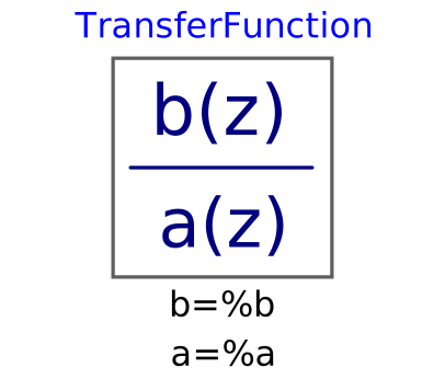
blockTransferFunction
Discrete-time Transfer Function block
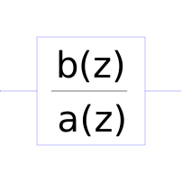
Extends from Modelica_Synchronous.RealSignals.Interfaces.PartialClockedSISO (Block with clocked single input and clocked single output Real signals).
Information
The discrete transfer function block defines the transfer function between the input signal u and the output signal y. The numerator has the order nb-1, the denominator has the order na-1.
          b(1)*z^(nb-1) + b(2)*z^(nb-2) + ... + b(nb)
   y(z) = -------------------------------------------- * u(z)
          a(1)*z^(na-1) + a(2)*z^(na-2) + ... + a(na)
State variables x are defined according to controller canonical form. Initial values of the states can be set as start values of x.
Example:
TransferFunction g(b = {2,4}, a = {1,3});
results in the following transfer function:
        2*z + 4
   y = --------- * u
         z + 3
Parameters
| Type | Name | Default | Description |
|---|---|---|---|
| Real[:] | b | {1} | Numerator coefficients of transfer function. |
| Real[:] | a | Denominator coefficients of transfer function. |
Connectors
| Type | Name | Default | Description |
|---|---|---|---|
| Modelica.Blocks.Interfaces.RealInput | u (from PartialClockedSISO) | Connector of clocked, Real input signal | |
| Modelica.Blocks.Interfaces.RealOutput | y (from PartialClockedSISO) | Connector of clocked, Real output signal |
Components
| Type | Name | Default | Description |
|---|---|---|---|
| Real[size(a, 1) - 1] | x | State vector of controller canonical form |
Revisions
Release Notes:
- August 13, 2012
by Bernhard Thiele:
Used the original code from Blocks.Discrete.TransferFunction and converted it into the Modelica 3.3 clocked equation style. - November 15, 2000
by Hans Olsson:
Converted to when-semantics of Modelica 1.4 with special care to avoid unnecessary algebraic loops. - June 18, 2000
by Martin Otter:
Realized based on a corresponding model of Dieter Moormann and Hilding Elmqvist.