packageKP07

Information

KP Scheme

Functions for solving PDEs in Modelica are described here. The Kurganov-Petrova (KP) scheme is a wellbalanced second-order scheme, which is a Riemann problem solver free scheme (central scheme) while at the same time, it takes advantage of the upwind scheme by utilizing the local, one side speed of propagation during the calculation of the flux at the cell interfaces.

Mathematical Formulation

The central-upwind numerical scheme is presented for the one-dimensional case:

$$ \frac{\partial U(x,t)}{\partial t} + \frac{\partial F(x,t,U)}{\partial x} = S(x,t,U) $$

where U(x,t) is the state vector, F(x,t,U) is the vector of fluxes and S(x,t,U) is the source terms.

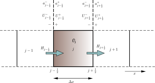
Figure: Control volume/cell for finite volume discretization.

Discretization

With the finite volume method, we divide the grid into small control volumes/cells and then apply the conservation laws. The semi-discrete (time-dependent ODEs) central-upwind scheme can be written as:

$$ \frac{\mathrm{d}}{\mathrm{d}t}\bar{U}_j(t) = -\frac{H_{j+\frac{1}{2}}(t) - H_{j-\frac{1}{2}}(t)}{\Delta x} + \bar{S}_j(t) $$

Here, Ū_j are the cell centre average values, while H_j±1/2(t) are the central upwind numerical fluxes at the cell interfaces. The numerical fluxes are calculated using the one-sided local speeds of propagation and the piecewise linearly reconstructed state values at cell interfaces.

Slope Limiter

The slope s_j of the reconstructed function in each cell is computed using a limiter function to obtain a non-oscillatory nature of the reconstruction. The KP scheme utilizes the generalized minmod limiter. The parameter θ ∈ [1,2] is used to control or tune the amount of numerical dissipation present in the resulting scheme. The value of θ = 1.3 is an acceptable starting point in general.

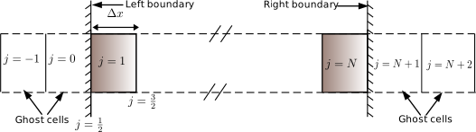
Figure: Ghost cells at the grid boundaries.

Ghost Cells

For boundary cells, imaginary cells called ghost cells are used outside the physical boundary. The average value of the conserved variables at the centre of these ghost cells depends on the nature of the physical boundary taken into account.

Implementation in OpenHPL

Functions for each element of the KP scheme are implemented in the KP07 package:

• GhostCells — provides values at ghost cells
• SlopeVectorS — returns the slope vector using the minmod limiter
• PieceWiseU — defines state values at cell interfaces
• SpeedPropagationApipe — provides one-sided local speeds of propagation
• FluxesH — defines central upwind numerical fluxes
• KPmethod — primary function that assembles all components

Note: Due to simulation speed considerations, these functions are implemented as model type instead of function type in OpenModelica.

Examples of using the KP scheme for solving PDEs are provided in class KP07. More information about using the KPmethod function is presented in the waterway modelling section for the PenstockKP and OpenChannel units.

Contents

Name	Description
KPmethod
KPfunctions
TestKPpde