Dynamic modeling of organic thermal systems is an highly challenging task. In order to enhance the performance and the robustness of the ThermoCycle library during initialization and integration different numerical methods have been implemented in the library. The adopted solutions are presented and discussed in this section.
Chattering
The phenomenon of chattering may occur when discontinuities in the model variables are present. This phenomenon can lead to extremely slow simulation, or to simulation failures because the computed variables exceed acceptable boundaries. In a discretized two-phase flow model, the main discontinuity is often the density derivative on the liquid saturation curve. Simulation failure or stiff systems can occur if the cell-generated (and purely numerical) flow rate due to this discontinuity causes a flow reversal in one of the nodes. Therefore, a numerical stability criteria can be expressed as follows:
Chattering and simulations failures are likely to occur if:
This section describes the different methods implemented to avoids the simulation issues described above. These methods aim at avoiding numerical flow reversal or avoiding unsolvable systems in case a flow reversal occurs. The different solutions are implemented and tested in the Modelica ThermoCycle library. Some can be implemented at the Modelica level while other require a modification of the thermodynamic properties of the working fluid. It should also be noted that some of these methods have already been proposed in the literature, while some others are new.
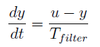
Filtering Method
In this strategy , a first order filter is applied to the fast variations of the density with respect to time:
where u and y are the input and output signals, respectively. In this particular case, u is the mass variation calculated with the equation of state and y is the filtered mass derivative. This filter therefore acts as ”mass damper” and avoids transmitting abrupt variations of the flow rate due the density derivative discontinuity. The filtered mass accumulation in each cell is written:
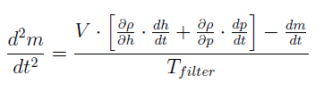
where Tfilter is the filter time constant, set as model input. This strategy displaces the mass variations in time but does not generate mass defects. However the energy balance is affected because the cell density is not exactly the one corresponding to the actual node flow rates. This approach is implemented at the model level, and can be activated by setting to true the filter_dMdt options in the Cell model, but it doubles the number of time states of the model since a second-order derivative of the working fluid mass is defined, as shown in the above equation.
Truncation method
This strategy acts on the partial derivative of density with respect to pressure and enthalpy. The peak in the density derivative occurring after the transition from liquid to two-phase is truncated. The maximum time derivative of the density is a model parameter and the maximum partial derivatives are calculated using the following equation:
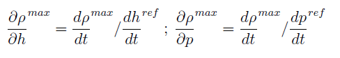
The reference values of the time derivatives of p and h are set to typical value. This allows for the use of a single parameter to compute the two maximum values of the partial derivatives. This strategy conserves mass balance in each cell, except when a phase transition occurs. In this case, a fictitious mass destruction appears. The underlying idea is that a mass defect is acceptable for the simulation if its value is limited and if it significantly increases the robustness of the model. This method is implemented at the model level and can be activated by the user by setting to true the max_der option in the Cell model.
Smoothing of the density derivative
The idea behind this method is to smooth out the density derivative discontinuity using a spline function. This can therefore only be performed at the level of the equation of state, i.e. in the thermophysical properties database. The open-source character of CoolProp allows to do so. The main drawback of this method is that the density function is still calculated with the original equation of state: smoothed derivative of density is not consistent with derivative from EOS. This might cause a mass defect during the simulation.
Smoothing of the density function
In order to avoid the mismatch between the density function and its derivative, one possible solution is to smooth the density for a range vapour qualities (i.e. making it C1-continuous) and recalculating its partial derivatives in the smoothed area. In this situation, the density derivatives are continuous but not smooth, which should still be manageable for the solver. The density is smoothed using a spline function with respect to the enthalpy between the liquid saturation line and a constant vapor quality line. The method is implemented in the standard distribution of CoolProp
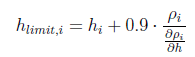
The enthalpy limiter method
The enthalpy limiter method does not aim at avoiding flow reversals. Instead, it ensures that the system of equations remains solvable even in case of flow reversal The enthalpy of the fluid entering a cell should have a minimum value, ensuring that the system of equations can be solved. The enthalpy limiter method is the practical implementation of this constraint in the cell model. It was originally proposed by Schultze et al. and implemented in the TIL Modelica library. The idea is to take profit of the ”Stream” connector type available in Modelica to propagate the minimum enthalpy limitation: in this manner a cell can communicate with its two neighbouring cell and propagate the minimum enthalpy of an incoming flow. The incoming flow is limited to this minimum value:
in the two adjacent cells, the enthalpy of the outlet flow is given by (example for i-1):
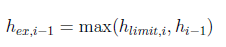
A security factor of 0.9 is taken to ensure a minimum distance between the outlet enthalpy and the theoretical limit. This method is implemented at the Modelica level and can be used by selecting the Cell1Dim_limit model.
Smooth Reversal Enthalpy
A discontinuity appears in the computed node enthalpy in case of flow reversal. This can be solved using a smooth transition between both parts of the equation. Eq. 2 is therefore transformed into:
![]()
The smooth transition is a C1-continuous sinusoidal transition function varying from 0 to 1 between - Mnom/10 and Mnom/10. Mnom is a user-defined model parameter. This method can be activeted by setting the Discretization scheme to UpWind with Smoothing in the Numerical option folder of the Cell1Dim model.