modelFresnelField
Fresnel field
Information
## Copyright © EDF 2002 - 2026
## ThermoSysPro Version 4.2
This component model is documented in Sect. 16.2 of the ThermoSysPro book.
# Fresnel field
The Linear Fresnel Reflector (LFR) is similar to the [parabolic trough collector](modelica://ThermoSysPro.Solar.Collectors.SolarCollector).
However, its receiver is not moving and thus made up of fewer moving parts.
This eliminates the need for strengthening materials.
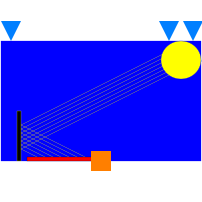
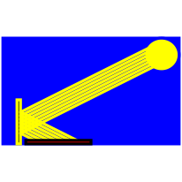
The LFR concentrates the solar radiation through long parallel rows of flat mirrors.
These modular mirrors focus the sunlight onto the receiver, which consists of a system of tubes through which the working fluid is pumped.
In addition, another mirror is placed above the absorber tube to reduce optical losses.
Flat mirrors allow more reflective surface in the same amount of space than a parabolic reflector, and they are much cheaper than parabolic reflectors.
## Modelica component model
The equations mentioned below are implemented in the component *FresnelField*, located in the *Solar.Collectors* sub-library.
This component has 5 connectors:
- Track: track input,
- SunG: azimuthal angle of the sun as function of time,
- SanA: elevation angle of the sun as function of time,
- SunDNI: solar radiation (Direct Normal Irradiance) as function of time,
- P: thermal power transfered to the fluid.

## Nomenclature
| Symbol| Description| Unit| Definition| Modelica name |
| :-------------------- | :------------------------------------------------------------------------ | :------------------------------------------- | :-------------------------------- | :-------------------------------- |
| \\(a\\)| Absorptivity of a train | \\(-\\)| 0.955| a |
| \\(A\\)| Area of all collectors| \\(\mathrm{m}^{2}\\)| | A |
| \\(D\\)| External pipe diameter \(absorber\)| \\(\mathrm{m}\\)| |D |
| \\(F\_{12}\\)| View factor to surroundings \(radiation heat loss\)| \\(-\\)| |F12 |
| \\(h\_{\mathrm{c}}\\)| Convective heat transfer coefficient between the ambient air and the pipe | \\(\mathrm{W} / \mathrm{m}^{2} / \mathrm{K}\\) | | hc |
| \\(K\_{\mathrm{L}}\\)| Longitudinal incidence angle modifier| \\(-\\)| | KL |
| \\(K\_{\mathrm{T}}\\)| Transversal incidence angle modifier| \\(-\\)| | KT |
| \\(L\\)| Length of a train | \\(\mathrm{m}\\) | \\(\frac{A}{w}\\)| L |
| \\(Lc\\)| Length of the collector| \\(\mathrm{m}\\) | \\(-\\)| Lc |
| \\(N\\)| Number of cells \(sections\) in the solar field| \\(-\\)| | Ns |
| \\(T\_{\text {atm }}\\)| Atmospheric temperature| \\(\mathrm{K}\\) | | T0 |
| \\(T\_{\mathrm{sky}}\\)| Sky temperature| \\(\mathrm{K}\\) | \\(0.0552 \cdot T\_{\text {atm }}^{1.5}\\) | 0.0552*T0^1.5 |
| \\(T\_{\mathrm{w}, i}\\)| Temperature of the outer receiver surface for cell \\(i\\)| \\(\mathrm{K}\\) | | T[i] |
| \\(w\\)| Aperture width of the collector| \\(\mathrm{m}\\) | | w |
| \\(W\_{\text {abs }}\\)| Solar radiation absorbed by the receiver| \\(\mathrm{W}\\) | | Qrec |
| \\(W\_{\mathrm{conv}, i}\\)| Convection power loss from the outer pipe surface to the ambient for cell \\(i\\)| \\(\mathrm{W}\\) | | |
| \\(W\_{\mathrm{rad}, i}\\)| Radiation power losses from the outer pipe surface to the ambient for cell \\(i\\)| \\(\mathrm{W}\\) | | |
| \\(W\_{\mathrm{t}, i}\\)| Thermal power transferred to the fluid for each cell \(section\) for cell \\(i\\)| \\(\mathrm{W}\\) | | dPth[i] |
| \\(z\\)| Height of the collector| \\(\mathrm{m}\\) | | h |
| \\(\alpha\_{\mathrm{s}}\\)| Sun elevation angle \(angle between the straight line to the sun and the horizontal plane\)| \\(^{\circ}\\)| | SunG0 |
| \\(\gamma\_{\mathrm{s}}\\)| Sun azimuth angle \(angle between the North and the solar position projected on the horizontal plane\) | \\(^{\circ}\\)| | SunA0 |
| \\(\varepsilon\_{\mathrm{t}}\\) | Tube emissivity| \\(-\\)| | emi |
| \\(\eta\_{\mathrm{av}}\\)| Mean availability of the solar field| \\(-\\)| \\(\le 1 \\)| dispo |
| \\(\eta\_{\mathrm{cl}}\\)| Mean cleanliness factor| \\(-\\) | \\( \le 1 \\) | clean |
|\\(\eta\_{\text {opt }}\\) | Optical efficiency at normal irradiation | \\(-\\) | | eta0 |
|\\(a\\) | Mean sun tracking system factor | \\(-\\) | \\(\leq 1\\) | track |
|\\(\theta\_{\mathrm{L}}\\) | Longitudinal incidence angle (angle between the zenith and the projection of the straight line to the sun onto the longitudinal plane "North-South") | \\(^{\circ}\\) | | thetaL|
|\\(\theta\_{\mathrm{T}}\\) | Transverse incidence angle (angle between the zenith and the projection of the straight line to the sun onto the transverse plane "North-South") | \\(^\circ\\) | | thetaT |
|\\(\rho\\) | Reflexivity of the primary reflector | \\(-\\) | \\(\approx 0.935\\) | rho |
|\\(\sigma\\) | Stefan-Boltzmann constant | \\(\mathrm{W} /\left\(\mathrm{m}^{2} \mathrm{K}^{4}\right\)\\) | \\(5.67 \times 10^{-8}\\) | 5.67e-8 |
|\\(\tau\\) | Transmissivity of the pipe wall | \\(-\\) | \\(\approx 0.965\\) | tau |
|\\(\phi\_{\text {sun }}\\) | Solar radiation (direct normal irradiance - DNI)| \\(\mathrm{W} / \mathrm{m}^{2}\\) | | DNI |
|\\(\chi\\) | Geometric default factor | \\(-\\) | | geo |
## Governing equations
### Thermal power received by the receiver
- Mathematical formulation:
$$W\_{\mathrm{rec}}=A \cdot \phi\_{\mathrm{sun}} \cdot \eta\_{\mathrm{opt}} \cdot K\_{\mathrm{T}} \cdot K\_{\mathrm{L}} \cdot \eta\_{\mathrm{av}} \cdot \eta\_{\mathrm{tr}} \cdot \eta\_{\mathrm{c} 1}$$
- Comments:
The optical efficiency at normal irradiation is given by
\\(\eta\_{\mathrm{opt}}=\rho \cdot a \cdot \tau \cdot \chi\\).
It is also possible for the user to directly provide a value for
\\(\eta\_{\mathrm{opt}}\\). <br/>
The polynomial function \\(K_T\\) is obtained by polynomial interpolation
based on the values obtained from Novatec Solar.
The transverse incidence angle
modifier is given by:
$$ K_{\mathrm{T}}= 3 \times 10^{-10} \cdot\left|\theta_{\mathrm{T}}\right|^{5}-5 \times 10^{-8} \cdot\left|\theta_{\mathrm{T}}\right|^{4}+1 \times 10^{-6} \cdot\left|\theta_{\mathrm{T}}\right|^{3} \\ -3 \times 10^{-5} \cdot\left|\theta_{\mathrm{T}}\right|^{2}-4 \times 10^{-4} \cdot\left|\theta_{\mathrm{T}}\right|+0.995$$
The longitudinal incidence angle modifier is given by
\\(K\_{\mathrm{L}}=\cos \left\(\theta\_{\mathrm{L}}\right\) \cdot\left\(1-\frac{z}{\mathrm{L}} \cdot \tan \left\(\theta\_{\mathrm{L}}\right\)\right\)\\).<br/>
The longitudinal incidence angle is given by \\(\theta\_{\mathrm{L}}=a \cdot \cos \(\sqrt{\left\(1-\cos ^{2}\left\(\alpha\_{\mathrm{s}}\right\) \cdot \cos ^{2}\left\(\gamma\_{\mathrm{s}}\right\)\right.}\)\\).<br/>
The transverse incidence angle is given by
$$ \theta_{\mathrm{T}}=\left\{\begin{array}{ll}90 \text{ for } \left|\sin \left(\alpha_{\mathrm{s}})| \leq 10^{-6}\right.\right. \\ \arctan \left(\frac{\sin (\gamma_{\mathrm{s}})}{\tan (\alpha_{\mathrm{s}})}\right) \text{ for }\left|\sin \left(\alpha_{s}) |>10^{-6}\right.\right.\end{array}\right.$$
### Energy balance equation for each cell (power transferred to the fluid)
- Mathematical formulation:
$$W\_{\mathrm{t}, i}=\frac{W\_{\mathrm{abs}}}{N}-W\_{\mathrm{rad}, i}-W\_{\mathrm{conv}, i}$$
- Comments:
The net power received by each tube segment is equal to the total power absorbed by the receiver for that segment minus the losses by radiation to the sky and convection to the ambient for that segment
### Radiation power losses
- Mathematical formulation:
$$W\_{\mathrm{rad} \mathrm{t}}=0.5 \cdot F\_{12} \cdot \sigma \cdot A\_{\mathrm{t}, i} \cdot \varepsilon\_{\mathrm{t}} \cdot\left\(T\_{\mathrm{w}, i}^{4}-T\_{\mathrm{sky}}^{4}\right\)$$
### Convection power losses to the ambient
- Mathematical formulation:
$$W\_{\text {conv }, i}=A\_{\mathrm{t}, i} \cdot h\_{\mathrm{c}} \cdot\left\(T\_{\mathrm{w}, i}-T\_{\mathrm{atm}}\right\)$$
- Comments:
\\(h\_{\mathrm{c}}\\) is given as input by the user.
## References
El Hefni, Baligh and Bouskela, Daniel (2019). [Modeling and Simulation of Thermal Power Plants with ThermoSysPro](https://link.springer.com/book/10.1007/978-3-030-05105-1), sect. 16.2. Springer Nature Switzerland AG.
Parameters
| Type | Name | Default | Description |
|---|
| Units.SI.Area | A | 10e4 | Aperture area of a train |
| Integer | mode_efficency | 1 | 1:Definition of each parameter : rho, a, tau , geo. 2:Definition of the global optical efficency |
| Real | eta0 | 0.625 | Global optical efficency at normal irradiation |
| Real | rho | 0.935 | Reflexivity of the primary reflector |
| Real | a | 0.955 | Absorptivity of the collector |
| Real | tau | 0.965 | Transmissivity of the glass envelope |
| Real | geo | 0.725 | Geometric default factor |
| Real | dispo | 1 | Mean disponibility of the field |
| Real | clean | 1 | Mean cleanliness factor |
| Units.SI.Length | h | 7.4 | Height of a collector |
| ThermoSysPro.Units.SI.Length | Lc | 44.8 | Length of a collector |
| Units.SI.Length | w | 11.46 | Aperture width of a collector |
| Units.SI.CoefficientOfHeatTransfer | hc | 1 | Heat transfer coefficient |
| Boolean | thermalLossPhy | true | true: thermal loss using a physical equation - false: thermal loss using a polynomial equation f(deltaT) |
| Units.SI.Diameter | D | 0.07 | External tube diameter (active if thermalLossPhy=true) |
| Real | F12 | 1 | View factor to surroundings radiation heat loss (active if thermalLossPhy=true) |
| Real | Emi | 0.8 | Tube emissivity (active if thermalLossPhy=true) |
| Real | A1 | 0.1598 | x coefficient of the linear thermal loss caracteristics Qloss=f(deltaT) (active if thermalLossPhy=false) |
| Real | A2 | 0.0057 | x^2 coefficient of the linear thermal loss caracteristics Qloss=f(deltaT) (active if thermalLossPhy=false) |
| Real | B0 | 0.995 | Constant coefficient of the KT caracteristics KT=f(thetaT) |
| Real | B1 | -4e-4 | x coefficient of the KT caracteristics KT=f(thetaT) |
| Real | B2 | -3e-5 | x^2 coefficient of the KT caracteristics KT=f(thetaT) |
| Real | B3 | 1e-6 | x^3 coefficient of the KT caracteristics KT=f(thetaT) |
| Real | B4 | -5e-8 | x^4 coefficient of the KT caracteristics KT=f(thetaT) |
| Real | B5 | 3e-10 | x^5 coefficient of the KT caracteristics KT=f(thetaT) |
| Real | B6 | 0 | x^6 coefficient of the KT caracteristics KT=f(thetaT) |
| Units.SI.Temperature | T0 | 300 | Atmospheric temperature |
| Integer | Ns | 10 | Number of cells (sections) in the field |
| ThermoSysPro.Units.nonSI.Angle_deg | SunA0 | 90 | Sun azimuth angle by default |
| ThermoSysPro.Units.nonSI.Angle_deg | SunG0 | 1e-6 | Sun elevation angle by default |
| Units.SI.Irradiance | SunDNI0 | 1000 | Direct normal irradiance by default |
| Real | trackingFactor | 1 | Mean sun tracking system factor |