
modelPseudoInversion1
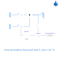
Extends from ThermofluidStream.Idealized.Tests.Inversion.BaseClasses.PartialInverse (Base model defining the mixing problem), Modelica.Icons.Example (Icon for runnable examples).
Information
This example demonstrates the mixing of two fluid streams, A and B, assuming constant specific heat capacities c_p.
The mixing equation is:
m_flow_A * T_A + m_flow_B * T_B = (m_flow_A + m_flow_B) * T_mix;
It can be easily solved for one unknown. This test demonstrates the "TFS way" of determining the mass flow rate
m_flow_B such that the mixing temperature T_mix = 25 °C.
Instead of using a nonlinear equation solver (e.g., Inversion1),
the TFS approach uses the time integration solver to solve the "nonlinear equation".
With a reasonable start value integrator.y_start and integrator gain integrator.k, the time integration solver will converge.
Specifically, convergence occurs for y_start >= 0, k > 0 or y_start < 0, k < 0, and divergence otherwise.
A larger integrator gain k results in faster convergence.
Mathematically, we introduce an auxiliary equation:
der(m_flow_B) = f(m_flow_B)
Because the time integrator is usually implicit, it also solves a nonlinear equation system:
m_flow_B_k+1 = m_flow_B_k + F(f(m_flow_B_k+1))
For example, using implicit Euler:
m_flow_B_k+1 = m_flow_B_k + dt * f(m_flow_B_k+1)
This effectively iterates in time. An explicit solver would limit the integrator gain k and is therefore not recommended
when aiming for high gains. In essence, this defines a custom algorithm for solving nonlinear equation systems.
The advantages of this approach are:
- Start values can be more explicitly defined than with, for example,
Inversion1. - The approach can handle limitations and resembles a model-based feed-forward control, instead of an explicit inversion
G⁻¹(s).
The disadvantages are:
- It introduces "pseudo" transients that might be undesirable.
- The time integration solver may have a lower convergence order. Step-size adaptive solvers may be strong, but using a controller essentially defines a custom nonlinear solver, which is usually less robust than established algorithms. Large gains or small time constants may result in stiff systems that are difficult to solve.
- The model-based feed-forward should ideally be stable, fast, without steady-state error, and should not introduce oscillations.
- It cannot produce an exact inverse model like
G⁻¹(s).
For design purposes, inversion is beneficial when only the quasi-stationary solution is sought. For dynamic simulations, especially with limitations, the model-based feed-forward approach can be very effective.
Components
| Type | Name | Default | Description |
|---|---|---|---|
| ThermofluidStream.DropOfCommons | dropOfCommons (from PartialInverse) | ||
| ThermofluidStream.Boundaries.Source | sourceA (from PartialInverse) | ||
| .ThermofluidStream.Idealized.Boundaries.Sink_free | sink (from PartialInverse) | ||
| ThermofluidStream.Idealized.Topology.JunctionT2 | junction (from PartialInverse) | ||
| ThermofluidStream.Boundaries.Source | sourceB (from PartialInverse) | ||
| .ThermofluidStream.Idealized.Boundaries.MassFlowRate | massFlowRateB (from PartialInverse) | ||
| .ThermofluidStream.Idealized.Boundaries.MassFlowRate | massFlowRateA (from PartialInverse) | ||
| ThermofluidStream.Sensors.SingleSensorSelect | singleSensorSelect (from PartialInverse) | ||
| Modelica.Blocks.Continuous.Integrator | integrator | ||
| Modelica.Blocks.Math.Feedback | feedback | ||
| Modelica.Blocks.Sources.RealExpression | temperatureSetpoint1 |
Revisions
-
2026, by Raphael Gebhart (raphael.gebhart@dlr.de):
Initial version.