This model simulates aquifer thermal energy storage, using one or multiple pairs of cold and hot wells.
To calculate aquifer temperature at different locations over time, the model applies physical principles of water flow and heat transfer phenomena. The model is based on the partial differential equation (PDE) for 1D conductive-convective transient radial heat transport in porous media
ρ c (∂ T(r,t) ⁄ ∂t) = k (∂² T(r,t) ⁄ ∂r²) - ρw cw u(∂ T(r,t) ⁄ ∂t),
where ρ is the mass density, c is the specific heat capacity per unit mass, T is the temperature at location r and time t, u is water velocity and k is the heat conductivity. The subscript w indicates water. The first term on the right hand side of the equation describes the effect of conduction, while the second term describes the fluid flow.
The pressure losses in the aquifer are calculated using the Darcy's law
Δp = ṁ g ⁄ (2 π K h ln(rMax ⁄ rWB)),
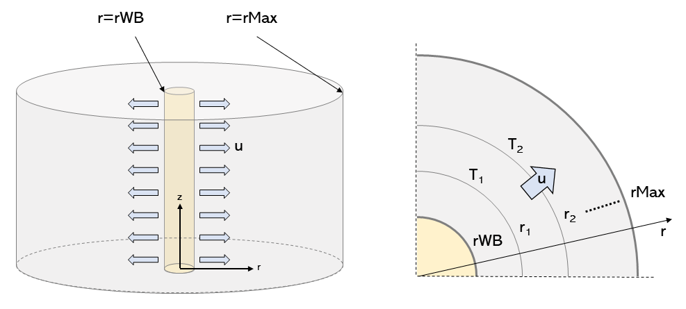
where ṁ is the water mass flow rate, g is the gravitational acceleration, K is the hydraulic conductivity, h is the thickness of the aquifer, rMax is the domain radius and rWB is the well radius. The pressure losses in the wells are calculated using Modelica.Fluid.Pipes.BaseClasses.WallFriction.Detailed.pressureLoss_m_flow.
To discretize the conductive-convective equation, the domain is divided into a series of thermal capacitances and thermal resistances along the radial direction. The implementation uses an array of Modelica.Thermal.HeatTransfer.Components.HeatCapacitor and Modelica.Thermal.HeatTransfer.Components.ThermalResistor. Fluid flow was modelled by adding a series of fluid volumes, which are connected to the thermal capacitances via heat ports. The fluid stream was developed using the model Buildings.Fluid.MixingVolumes.MixingVolume. The geometric representation of the model is illustrated in the figure below.
By default, the component consists of a single pair of wells:
one cold well and one warm well. The number of paired wells can be
increased by modifing the parameters nPai. The effect
is a proportional increase of thermal capacity, and the mass flow
rate at port_a and port_b is equally
distributed to the pairs of well, thus all pairs have the same mass
flow rates and temperatures, and the quantities at the fluid ports
is for all well combined, as is the electricity consumption
PTot for the well pumps.
To ensure conservation of energy, the wells are connected via
fluid ports. To avoid thermal interferences, make sure that the
aquifer domain radius rMax is large enough for your
specific use case.
Circulation pumps are included in the model and they can be
controlled by acting on the input connector. The input must vary
between [1, -1]. A positive value will circulate water
clockwise (from port_Hot to port_Col,
thus extraction from the cold well and injection into the warm
well). A negative value will circulate water anticlockwise.
The temperature values in the warm and cold aquifers can be
accessed using TAquHot and TAquCol. These
temperatures correspond to the temperatures of each thermal
capacitance in the discretized domain. The location of the thermal
capacitance is expressed by rVol.
The model computes the flow resistance of the cold well and the cold acquifer. Because of symmetry, the warm side has the same flow resistances. To reduce the number of equations in the model, the flow resistance of the warm side is set to the same flow resistance as on the cold side, but with the sign reversed.
| Name | Description |
|---|---|
| Medium in the component |