This model calculates the ground temperature response to obtain the temperature at the borehole wall in a geothermal system where heat is being injected into or extracted from the ground.
A load-aggregation scheme based on that developed by Claesson
and Javed (2012) is used to calculate the borehole wall temperature
response with the temporal superposition of ground thermal loads.
In its base form, the load-aggregation scheme uses fixed-length
aggregation cells to agglomerate thermal load history together,
with more distant cells (denoted with a higher cell and vector
index) representing more distant thermal history. The more distant
the thermal load, the less impactful it is on the borehole wall
temperature change at the current time step. Each cell has an
aggregation time associated to it denoted by
nu, which corresponds to the simulation time (since
the beginning of heat injection or extraction) at which the cell
will begin shifting its thermal load to more distant cells. To
determine nu, cells have a temporal size
rcel (rcel in this model) which
follows the exponential growth
where nCel is the number of consecutive cells
which can have the same size. Decreasing rcel
will generally decrease calculation times, at the cost of precision
in the temporal superposition. rcel is expressed in
multiples of the aggregation time resolution (via the parameter
tLoaAgg). Then, nu may be expressed as
the sum of all rcel values (multiplied by the
aggregation time resolution) up to and including that cell in
question.
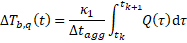
To determine the weighting factors, the borefield's temperature step response at the borefield wall is determined as
where g(·) is the borefield's thermal response factor
known as the g-function, H is the total length of
all boreholes and ks is the thermal conductivity
of the soil. The weighting factors kappa (κ in
the equation below) for a given cell i are then expressed as
follows.
where ν refers to the vector nu in this
model and Tstep(ν0)=0.
At every aggregation time step, a time event is generated to perform the load aggregation steps. First, the thermal load is shifted. When shifting between cells of different size, total energy is conserved. This operation is illustred in the figure below by Cimmino (2014).
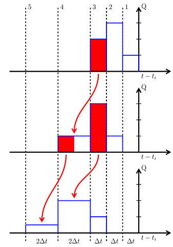
After the cell-shifting operation is performed, the first
aggregation cell has its value set to the average thermal load
since the last aggregation step. Temporal superposition is then
applied by means of a scalar product between the aggregated thermal
loads QAgg_flow and the weighting factors
κ.
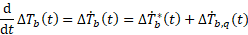
Due to Modelica's variable time steps, the load aggregation scheme is modified by separating the thermal response between the current aggregation time step and everything preceding it. This is done according to
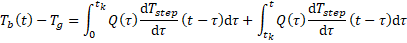
where Tb is the borehole wall temperature,
Tg is the undisturbed ground temperature,
Q is the ground thermal load per borehole length and h =
g/(2 π ks) is a temperature response factor based on
the g-function. tk is the last discrete
aggregation time step, meaning that the current time t
satisfies tk≤t≤tk+1.
Δtagg(=tk+1-tk) is the
parameter tLoaAgg in the present model.
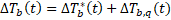
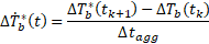
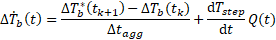
Thus, ΔTb*(t) is the borehole wall temperature change due to the thermal history prior to the current aggregation step. At every aggregation time step, load aggregation and temporal superposition are used to calculate its discrete value. Assuming no heat injection or extraction until tk+1, this term is assumed to have a linear time derivative, which is given by the difference between ΔTb*(tk+1) (the temperature change from load history at the next discrete aggregation time step, which is constant over the duration of the ongoing aggregation time step) and the total temperature change at the last aggregation time step, ΔTb(t).
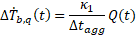
The second term ΔTb,q(t) concerns the ongoing
aggregation time step. To obtain the time derivative of this term,
the thermal response factor h is assumed to vary linearly
over the course of an aggregation time step. Therefore, because the
ongoing aggregation time step always concerns the first aggregation
cell, its derivative (denoted by the parameter
dTStepdt in this model) can be calculated as
kappa[1], the first value in the kappa
vector, divided by the aggregation time step Δt. The
derivative of the temperature change at the borehole wall is then
expressed as the multiplication of dTStepdt (which
only needs to be calculated once at the start of the simulation)
and the heat flow Q at the borehole wall.
With the two terms in the expression of ΔTb(t)
expressed as time derivatives, ΔTb(t) can itself
also be expressed as its time derivative and implemented as such
directly in the Modelica equations block with the
der() operator.
This load aggregation scheme is validated in Buildings.Fluid.Geothermal.Borefields.BaseClasses.HeatTransfer.Validation.Analytic_20Years.
Cimmino, M. 2014. Développement et validation expérimentale de facteurs de réponse thermique pour champs de puits géothermiques, Ph.D. Thesis, École Polytechnique de Montréal.
Claesson, J. and Javed, S. 2012. A load-aggregation method to calculate extraction temperatures of borehole heat exchangers. ASHRAE Transactions 118(1): 530-539.
Prieto, C. and Cimmino, M. 2021. Thermal interactions in large irregular fields of geothermal boreholes: the method of equivalent boreholes. Journal of Building Performance Simulation 14(4): 446-460. doi:10.1080/19401493.2021.1968953.
when block to avoid continuous and
discrete variable assignment in the same block.