.IdealizedContact.ContactBlock.Contact

Information

Depending on the shape, we use 1 (sphere), 2 (cylinder) or 4 (plane) points to describe the surfaces of the contact partners. These constitute potential contact points. For each of them the collision detection is performed. For this purpose, analytic solutions for simple geometries are provided in the library. As the contact region may alter with the moving bodies, the contact points will also move on the defined surface.

Then, the contact block calculates the appropriate force depending on the combination of surfaces. So, using it the respective combination of contact surface has to be chosen at first by setting the parameter contactDefinition. This will use the Modelica replaceable statement to define the appropiate components of the contact block. Then connect the contact interfaces of the two contact surfaces to the respective port of the contact block (first surface mentioned must be connected to port 1).

In the case of a collision of the two connected surface (the contact condition holds for at least one contact point) a three-dimensional contact force is applied. It consists of both the normal force and the tangential friction. The respective directions can be obtained by means of the local coordinate systems in the contact points. As compared to more complex models, the continuous surface layer is replaced by a nonlinear spring/damper element. Consequently, the normal force Fn is determined by means of the penetration p and the penetration velocity. A continuous contact force model with hysteresis damping according to [1] is implemented. Nevertheless, choosing n1=1 and n=0 one can get the linear Kelvin-Voigt model, where the coefficients are the spring and damping constant. Choosing n1=n2 one will get the formulation according to [2].

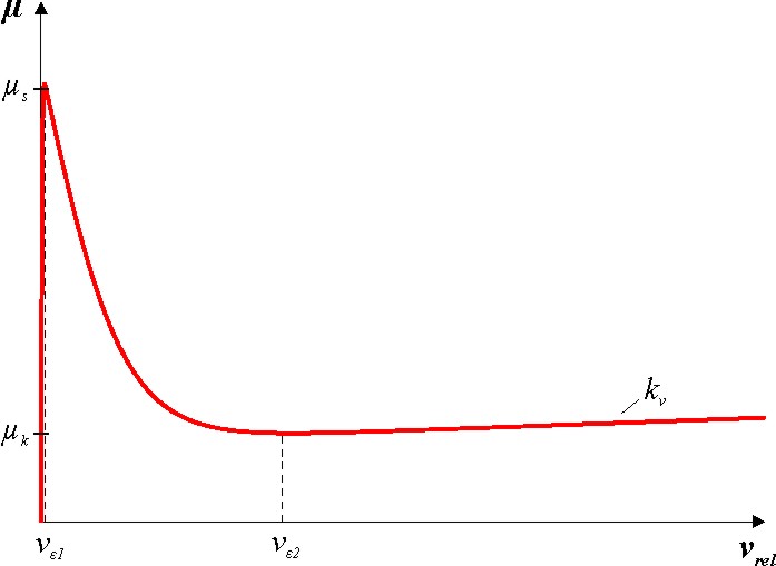
In order to calculate the friction forces without further discontinuous events, which would decrease the simulation speed and impede controller design, we use the continuously differentiable friction model of Makkar et al. [3]. They introduced the following function of the relative velocity to approximate the friction coefficient of the characteristic Stribeck curve.

In doing so, no ideal static friction can be obtained because the actual force to be applied in the static state is independent from the relative velocity of the two bodies. Static friction is rather represented by sliding with very small relative velocities. To set the unknown constants gamma_i we use five parameters, which can be seen in the figure. The parameters mue_s and mue_k denote the coefficients of static and kinetic friction. The limit velocity v_e1 and v_e2 define the beginning of mixed and viscous friction. The latter is described by the proportionality factor k_v. The actual approximation can be monitored by calling the function plotFrictionCurve.

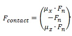
The complete vector of the contact force is then computed as follows.

Note: The collision of two cylinders can lead to linear or punctiform contact regions. The calculation for these two cases is currently seperated in two blocks. Integration of the two blocks is in progress.

References:

[1]          H. M. Lankarani, P. E. Nikravesh: Continuous Contact Force Models for Impact Analysis in Multibody Systems, Nonlinear Dynamics, 5, 1994

[2]          K. H. Hunt, F. R. E. Crossley: Coefficient of restitution interpreted as damping in vibroimpact, ASME J. Appl. Mech, 1975

[3]          C. Makkar, W. E. Dixon, W. G. Sawyer, G. Hu: A New Continuously Differentiable Friction Model for Control Systems Design, Proceedings of the 2005 IEEE/ASME International Conference on Advanced Intelligent Mechatronics, Monterey CA, July, 2005