This example demonstrates how to construct an inverse model in Modelica (for more details see Looye, Thümmel, Kurze, Otter, Bals: Nonlinear Inverse Models for Control).
For a linear, single input, single output system
y = n(s)/d(s) * u // plant model
the inverse model is derived by simply exchanging the numerator and the denominator polynomial:
u = d(s)/n(s) * y // inverse plant model
If the denominator polynomial d(s) has a higher degree as the numerator polynomial n(s) (which is usually the case for plant models), then the inverse model is no longer proper, i.e., it is not causal. To avoid this, an approximate inverse model is constructed by adding a sufficient number of poles to the denominator of the inverse model. This can be interpreted as filtering the desired output signal y:
u = d(s)/(n(s)*f(s)) * y // inverse plant model with filtered y
With Modelica it is in principal possible to construct inverse models not only for linear but also for non-linear models and in particular for every Modelica model. The basic construction mechanism is explained at hand of this example:
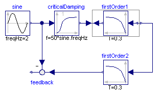
Here the first order block "firstOrder1" shall be inverted. This is performed by connecting its inputs and outputs with an instance of block Modelica.Blocks.Math.InverseBlockConstraints. By this connection, the inputs and outputs are exchanged. The goal is to compute the input of the "firstOrder1" block so that its output follows a given sine signal. For this, the sine signal "sin" is first filtered with a "CriticalDamping" filter of order 1 and then the output of this filter is connected to the output of the "firstOrder1" block (via the InverseBlockConstraints block, since 2 outputs cannot be connected directly together in a block diagram).
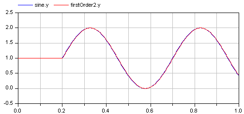
In order to check the inversion, the computed input of "firstOrder1" is used as input in an identical block "firstOrder2". The output of "firstOrder2" should be the given "sine" function. The difference is constructed with the "feedback" block. Since the "sine" function is filtered, one cannot expect that this difference is zero. The higher the cut-off frequency of the filter, the closer is the agreement. A typical simulation result is shown in the next figure: