.Modelica_LinearSystems2.TransferFunction.Plot.initialResponse

Information

Syntax

TransferFunction.Plot.initialResponse(tf)
   or
TransferFunction.Plot.initialResponse(
  tf,
  dt,
  tSpan,
  y0,
  columnLabels,
  defaultDiagram=Modelica_LinearSystems2.Internal.DefaultDiagramTimeResponse(),
  device=Modelica_LinearSystems2.Utilities.Plot.Records.Device())

Description

This function plots the initial response, i.e. the zeros input response of a transfer function. It is based on timeResponse.

Example

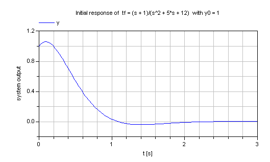
  TransferFunction s = Modelica_LinearSystems2.TransferFunction.s();
  Modelica_LinearSystems2.TransferFunction tf = (s + 1)/(s^2 + 5*s + 12);
  Real y0=1;

algorithm
  Modelica_LinearSystems2.TransferFunction.Plot.initialResponse(tf,y0=y0, dt=0.02, tSpan=3)
//  gives:

See also

impulse, step, ramp

Interface

encapsulated function initialResponse
  import Modelica;
  import Modelica_LinearSystems2;
  import Modelica_LinearSystems2.TransferFunction;
  import Modelica_LinearSystems2.Utilities.Types.TimeResponse;
  import Modelica_LinearSystems2.Utilities.Plot;
  input Modelica_LinearSystems2.TransferFunction tf;
  input Real dt = 0 "Sample time [s]";
  input Real tSpan = 0 "Simulation time span [s]";
  input Modelica_LinearSystems2.Utilities.Types.TimeResponse response = Modelica_LinearSystems2.Utilities.Types.TimeResponse.Initial "type of time response";
  input Real y0 "Initial output (for initial condition plot)";
  extends Modelica_LinearSystems2.Internal.PartialPlotFunction(defaultDiagram = Modelica_LinearSystems2.Internal.DefaultDiagramTimeResponse(heading = "Initial response of  tf = " + String(tf) + "  with y0 = " + String(y0)));
end initialResponse;