.Modelica_Synchronous.RealSignals.Sampler.Sample

Information

This block samples the continuous-time, Real input signal u and provides it as clocked output signal y. The clock of the output signal is inferred (that is, it needs to be defined somewhere else in the clocked partition). If this is not desired, use block SampleClocked instead, to explicitly assign a clock to the output signal.

To be more precise: The input signal u(t) must be a continuous-time signal. The output signal y(ti) is associated to a clock (defined somewhere else). At a clock tick, the left limit of u is assigned to y: y(ti) = u(ti-eps) (= the value of u just before the clock became active). Since the operator returns the left limit of u, it introduces an infinitesimal small delay between the continuous-time and the clocked partition. This corresponds to the reality, where a sampled data system cannot act infinitely fast and even for a very idealized simulation, an infinitesimal small delay is present. As a result, algebraic loops between clocked and continuous-time partitions cannot occur.

Examples

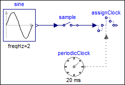
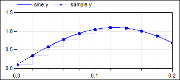
The following example samples a sine signal with a periodic clock of 20 ms period:

	model	simulation result

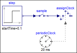
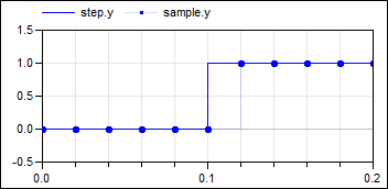
In the following example the continuous-time input signal contains a discontinuous value change at the 0.1 s clock tick. It can be seen that the Sample block samples the left limit of the step signal:

	model	simulation result

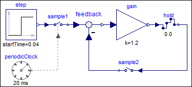
In the following example a direct feedthrough in the continuous-time and in the clocked partition is present. Without a time-delay, this would result in an algebraic loop. However, since block Sample samples the left limit of a continuous-time signal, sampling introduces a delay of one sample period that breaks the algebraic loop:

	model
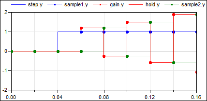
	simulation result

Note, the reason for the delay is that sample2.y (= the green, clocked signal) is the left limit of hold.y (= the red, continuous-time signal).