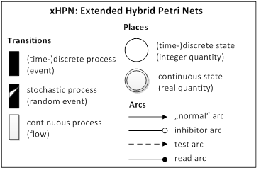
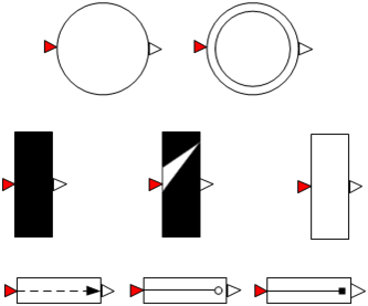
The xHPN formalism comprises of three different processes, called transitions: discrete, stochastic, and continuous transition, two different states, called places: discrete and continuous places, and four different arcs: normal, inhibition, test, and read arc. The icons of the formalism are shown in the following figure.
Discrete places contain an integer quantity, called tokens or marks while continuous places contain a non-negative real quantity. These marks initiate transitions to fire according to specific conditions. These firings lead to changes of the marks in the connected places.
Discrete transitions are provided with delays and firing conditions and fire first when the associated delay is passed and the conditions are fulfilled. These fixed delays can be replaced by exponentially distributed random values, then, the corresponding transition is called stochastic transition. Thereby, the characteristic parameter λ of the exponential distribution can depend functionally on the markings of several places and is recalculated at each point in time when the respective transition becomes active or when one or more markings of involved places change. Based on the characteristic parameter, the next putative firing time τ=time+Exp(λ) of the transition can be evaluated and it fire when this point in time is reached.
Both - discrete and stochastic transitions - fire by removing the arc weight from all input places and adding the arc weight to all output places. On the contrary, the firing of continuous transitions takes places as a continuous flow determined by the firing speed which can depend functionally on markings and/or time.
Places and transitions are connected by normal arcs which are weighted by integer and non-negative real numbers, respectively. But also functions can be written at the arcs depending on the current markings of the places and/or time. Places can also be connected to transitions by test, inhibition, and read arcs. Then their markings do not change during the firing process. In the case of test and inhibitor arcs, the markings are only read to influence the time of firing while read arcs only indicate the usage of the marking in the transition, e.g. for firing conditions or speed functions.
If a place is connected to a transition by a test arc, the marking of the place must be greater than the arc weight to enable firing. If a place is connected to a transition by an inhibitor arc, the marking of the place must be less than the arc weight to enable firing. In both cases the markings of the places are not changed by fining.
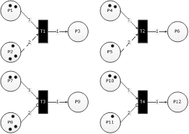
The Petri nets at top contain test arcs and the Petri nets at the bottom inhibitor arcs. Transition T1 is active with regard to a concrete marking m because the token number of P2 is above the weight of the test arc (m(P2)=3>f(P2→T1)=2). However, T2 is not active because the marking of P5 is less than the arc weight (m(P5)=1<f(P5→T2)=2). T3 is also not active because the token number of P8 is greater than the weight of the inhibitor arc (m(P8)=3>f(P8→T3)=2). However, T4 is active because the marking of P11 is less than the arc weight (m(P11)=1<f(P11→T4)=2).
The conversion of a discrete to a continuous marking is realized by connecting a discrete transition to a continuous place and the conversion from a continuous to a discrete marking is realized by connecting a continuous place to a discrete transition. However, the conversion is always performed by discrete transitions, discrete places can only influence the time when continuous transitions fire but their marking cannot be changed during the firing process.
The figure shows examples of these two basic principles:
It is important to mention that a discrete transition fires always in a discrete manner by removing and adding marks after a delay is passed regardless of whether a discrete or a continuous place is connected to it. However, a continuous transition fires always by a continuous flow so that a discrete place can only be connected to continuous transition if it is input as well as output of the transition with arcs of same weight. In this way the continuous transition can only be influenced by a discrete place but the discrete marking cannot be changed by continuous firing.
Summarized, an xHPN comprises of:
A formal definition of the xHPN-formalism and the corresponding processes is given in [Proß et al.2012].
Several conflicts can occur when the places have to enable their connected active transitions. Possibly, a discrete place or a continuous place connected to discrete transitions has not enough marks to enable all output transitions simultaneously or cannot receive marks from all active input transitions due to the maximum capacity. Then an actual conflict arises that has to be resolved. This can be either done by providing the transitions with priorities or probabilities. In the first case, a deterministic process decides which place enables which transitions and in the second case the enabling is performed at random; thereby transitions assigned with a high probability are chosen preferentially.
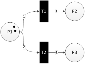
Both transitions of the Petri net example are active because
of
m(P1)=2≥f(P1→T1)=1
and
m(P1)=2≥f(P1&arr;T2)=2.
But P1 can only enable one of them due to its token number. Hence,
P1 has a actual conflict. If the enabling is performed by
priorities and T2 has priority 1 and T1 has priority 2, P1 enables
T2. T2 is firable and fires by removing two tokens from P1 and
adding one to P3. If the enabling is performed at random, one of
the transitions is enabled according to their assigned
probabilities, e.g. T1 has the probability 0.7 and T2 has the
probability 0.3.
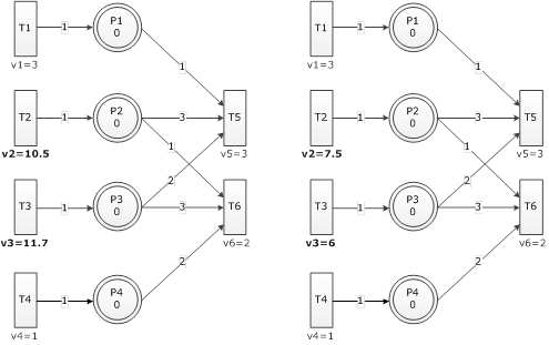
Another conflict can occur between a continuous place and two or more continuous transitions when the input speed is not sufficient to fire all output transitions with the instantaneous speed (type-2-output-conflict) or when the output speed is not sufficient to fire all input transitions with the instantaneous speed (type-2-input-conflict). This conflict is solved by sharing the speeds proportional to the assigned maximum speeds (see [Proß2012]).
The left Petri net has no actual conflict but P2 and P3 of the right Petri net have an actual conflict. Their input speed is not sufficient to fire T5 and T6 with the respective speed.
If a conflict occurs between a place and continuous as well as discrete/stochastic transitions, the discrete/stochastic transitions take always priority over the continuous transitions.
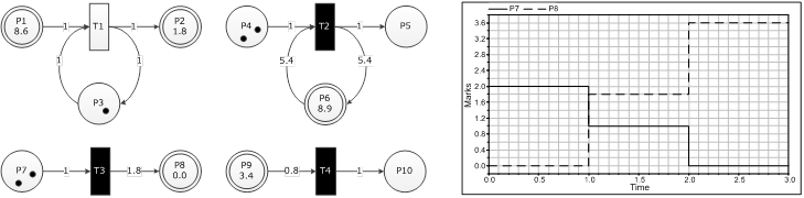
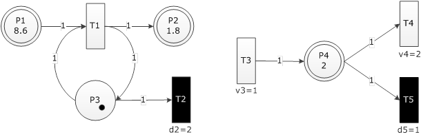
The figure shows two examples of type-3-conflicts. At time 0, transition T1 of the left Petri net becomes active and fires continuously. At time 2, the delay of T2 is passed and it becomes firable. At this point in time, P3 has an actual conflict because it cannot fire token in T1 and T2, simultaneously. Hence, T2 takes priority over T1 and fires. At time 0, transitions T3 and T4 of the right Petri net fire continuously. At time 1, m(P4)=1 and the delay of T5 is passed; hence, P4 has an actual conflict. The conflict only occurs when the marking equals the arc weight. If m(P4)<f(P4→T5) or m(P4)>f(P4→T5), there is no conflict. It is solved by the rule that T5 takes priority over T4 and fires. This rule is intuitively logical because the firing of a continuous transition is a continuous flow and the firing of a discrete transition is an extreme change of the Petri net marking.
A last conflict can occur when a discrete place has not enough marks to enable all connected continuous transitions. This is solved by prioritization of the involved transitions.
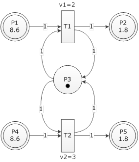
The figure shows a hybrid Petri net; place P3 has a type-4-conflict. At time 0, P3 can either activate T1 or T2 but not both simultaneously. This conflict can be solved by prioritization of the transitions. If T1 takes priority over T2, T1 becomes active and fires and if T2 takes priority over T1, T2 becomes active and fires. Therefore, all continuous output transitions of a discrete place have to be provided with priorities.
Compatibility
The advanced Petri Net library, called PNlib, enables the modeling of extended hybrid Petri Nets (xHPN). It comprises
The main package PNlib is divided into the following sub-packages:
Additionally, the package contains the component settings which enables the setting of global parameters for the display and animation of a Petri net model:
Places, transitions, and arcs are represented by the icons depicted in the figure. Thereby, the discrete place is represented by a circle and the continuous place by a double circle. The transitions are boxes which are black for discrete transitions, black with a white triangle for stochastic transitions, and white for continuous transitions. The test arc is represented by a dashed arc, the inhibitor arc by an arc with a white circle at its end, and the read arc by an arc with a black square at its end.
The PNlib contains four different connectors: PlaceOut, PlaceIn, TransitionOut, and TransitionIn. The connectors PlaceOut and PlaceIn are part of place models and connect them to output and input transitions, respectively. Similar, TransitionOut and TransitionIn are connectors of the transition model and connect them to output and input places, respectively. The figure shows which connector belongs to with Petri net component model.
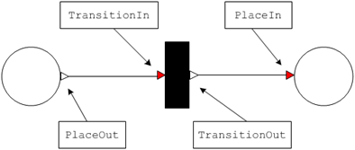
The connectors of the Petri net component models are vectors to enable the connection to an arbitrary number of input and output components. Therefore, the dimension parameters nIn and nOut are declared in the place and transition models with the connectorSizing annotation.
Parameters and modification possibilities of discrete (d) and continuous (c) places:
| Name | Type | Default | Allowed | Description |
|---|---|---|---|---|
| startTokens/startMarks | scalar | 0 | integers (d)/positive real values (c) | Marking at the beginning of the simulation |
| minTokens/minMarks | scalar | 0 | integers (d)/positive real values (c) | Minimum capacity |
| maxTokens/maxMarks | scalar | infinite | integers (d)/positive real values (c) | Maximum capacity |
| enablingType | choice/scalar | Priority | priority or probability | Type of enabling if type-1-conflicts occur; the priorities are defined by the connection indices and the probabilities by the variables enablingProbIn/Out |
| enablingProbIn | vector | fill(1/nIn, nIn) | sum must be equal to one | Enabling probabilities of input transitions |
| enablingProbOut | vector | fill(1/nOut, nOut) | sum must be equal to one | Enabling probabilities of output transitions |
| N | scalar | settings.N | integers (d) | Amount of levels for stochastic simulation |
| reStart | condition expression | false | Boolean condition expression | Condition for resetting the marking to reStartTokens/Marks |
| reStartTokens/reStartMarks | scalar | 0 | integers (d)/positive real values (c) | when the reStart condition is fulfilled, the marking is set to reStartTokens/Marks |
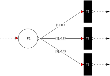
If the type-1-conflict is resolved by priorities, the corresponding priorities of the transitions are given by the indices of the connections, i.e. the transition connected to the place with the index 1 has also the priority 1, the transition connected to the place with the index 2 has also the priority 2 etc. Otherwise, if the probabilistic enabling type is chosen, the corresponding probabilities for the transitions have to be entered as a vector (numbers separated by commas within braces). Thereby, the first vector element corresponds to the connection with the index 1, the second to the connection with the index 2 etc. The input of enabling probabilities as vectors in the place model, and not at the corresponding arcs, is necessary due to the fact that properties cannot be assigned to connections according to the Modelica Specification 3.2.
Place P1 is connected to the transitions T1, T2, and T3 and the connection to T1 is indexed by 1, the connection to T2 is indexed by 2, and the connection to T3 is indexed by 3. Thus, the corresponding connect-equations are connect(P1.outTransition[1], T1.inPlaces[1]); connect(P1.outTransition[2], T2.inPlaces[1]); connect(P1.outTransition[3], T3.inPlaces[1]); The enabling probabilities 0.3 for T1, 0.25 for T2, and 0.45 for T3 have to be entered by the parameter vector enablingProbOut={0.3, 0.25, 0.45}.
The main process in the place model is the recalculation of the marking after firing a connected transition. In the case of the discrete place model, this is realized by the discrete equation
when tokeninout or pre(reStart) then
  t = if tokeninout then pre(t) + firingSumIn - firingSumOut else reStartTokens;
end when;
whereby pre(t) accesses the marking t immediately before the transitions fire. To this amount, the arc weight sum of all firing input transitions is added and the arc weight sum of all firing output transitions is subtracted from it. Additionally, the tokens are reset to reStartTokens when the user-defined condition reStart becomes true.
The marking of continuous places can change continuously as well as discretely. This is implemented by the following construct
der(t) = conMarkChange;
when disMarksInOut then
  reinit(t, t + disMarkChange);
end when;
when reStart then
  reinit(t, reStartMarks);
end when;
whereby the der-operator access the derivative of the marking t according to time. The continuous mark change is performed by a differential equation while the discrete mark change is performed by the reinit-operator within a discrete equation. This operator causes a re-initialization of the continuous marking every time when a connected discrete transition fires. Additionally, the marking is re-initialized by reStartMarks when the condition reStart becomes true.
Parameters and modification possibilities of discrete (d), stochastic (s), and continuous (c) transitions
| Name | Type | Part of | Default | Allowed | Description |
|---|---|---|---|---|---|
| delay | scalar | d | 1 | positive real values | Delay of timed transitions |
| h | scalar or scalar function | s | 1 | positive real values | Hazard function to determine the characteristic value of exponential distribution |
| maximumSpeed | scalar or scalar function | c | 1 | positive real values | Maximum speed |
| arcWeightIn | vector or vector function | d, s, c | fill(1, nIn) | integers (d, s) positive real values (c) | Weights of input arcs |
| arcWeightOut | vector or vector function | d, s, c | fill(1, nOut) | integers (d, s) positive real values (c) | Weights of output arcs |
| firingCon | condition expression | d, s, c | true | Boolean condition expression | Firing condition |
It has to be distinguished between the following input types: scalar, vector, scalar function, vector function, and condition expression. The input of the different types is demonstrated by the examples. The input of arc weights as vectors in the transition model and not at the respective arcs is necessary due to the fact that connections cannot be provided with properties according to the Modelica Specification 3.2.
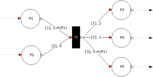
The figure shows a discrete Petri net. The indices of the connections are written at the arcs within square brackets, e.g. the connection (P1-T1) has the input index [1] and (T1-P5) has the output index [3]. The input of the arc weights displayed after the indices to property dialog or as modification equation is performed by the vector functions
arcWeightIn = {2*P1.t, 4} and arcWeightOut = {2, 1, 5*P1.t},
whereby the expression P1.t accesses the current token number of P1. Thus, the weights of the arcs (P1-T1) and (T1-P5) are functions which depend on the token number of P1. Transitions can also be provided with additional conditions that have to be satisfied to permit the activation. The condition
firingCon = time > 9.7
causes that the transition cannot be activated as long as time is less than 9.7.
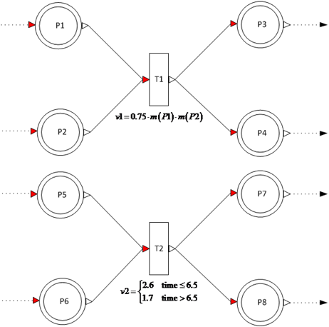
The figure shows two continuous Petri nets. Transition T1 has a maximum speed function which depends on the makings of P1 and P2. The input of this function to the property dialog or as modification equation is performed by the expression
maximumSpeed = 0.75*P1.t*P2.t,
whereby P1.t and P2.t accesses the marks of P1 and P2, respectively. Transition T2 has a maximum speed function that depends on time and can be entered by the expression
maximumSpeed = if time≤6.5 then 2.6 else 1.7.
Based on the current markings of the places, it is checked in the transition model by an algorithmic procedure if the transition can become active. discrete transition waits then as long as the delay is passed and a stochastic transition waits till the next putative firing time is reached. Based on this information the places enable some of the active transition to fire. At this point, several conflicts can occur which have to be resolved appropriately by the methods mentioned in [Proß2012] to get a successful and reliable simulation. When a transition is enabled by all its connected places, it is firable and reports this via the connector variable fire to the connected places. The places recalculate then their markings based on this information.
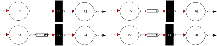
xHPNs comprise four different kinds of arcs: normal, test, inhibitor, and read arc. The Modelica language do not support the assignment of properties to arcs that are generated by connect equations. Due to that fact, the test, inhibitor, and read arcs are realized by component models which are interposed between places and transitions (see figure); the normal arc is simply generated by the connect equation. Test and inhibitor arc can be normal arcs simultaneously.
Parameters of test and inhibitor arcs (read arcs have no parameters)
| Name | Type | Default | Allowed | Description |
|---|---|---|---|---|
| testValue | scalar | 1 | integers if connected to discrete places, positive real values if connected to continuous places | The marking of the place must be greater to enable firing of transitions (test arc), marking of the place hat to be smaller to enable firing (inhibitor arc) |
| normalArc | choice/scalar | no | no or yes | If yes is chosen then is the arc also a normal arc to change the marking by firing (called double arc) |
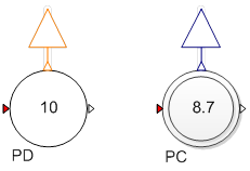
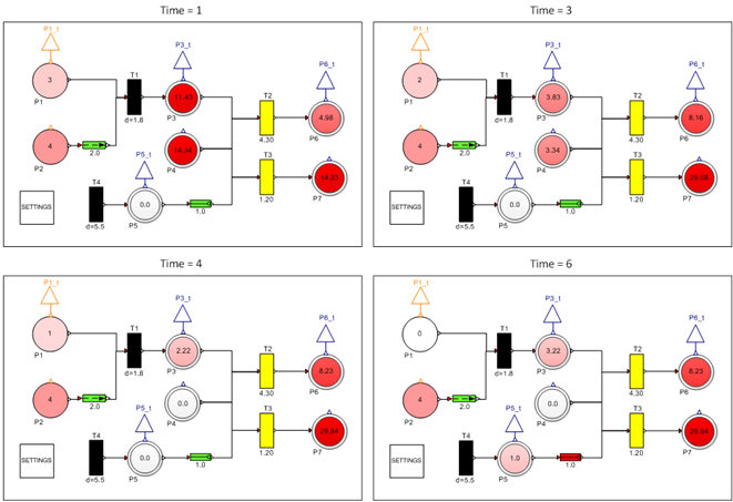
A possibility to represent the simulation results of an xHPN model is an animation. Thereby, several settings can be made in the property dialog of the settings-box. These settings are global and, thus, affect all components of the Petri net model. By using the prefixes inner and outer, it is achieved that the settings are common to all Petri net components of a model. The settings-box provides several display and animation options mentioned before. The animation toolbar allows the control of the animation. An animation offers a way to analyze the marking evolutions of large and complex xHPNs. The figure shows four selected points in time of the animation of an xHPN example.
All display and animation options are realized with the DynamicSelect annotation.
To simulate the established xHPN model several times with different parameter settings and use the arising simulation results for parameter estimation, sensitivity analysis, deterministic and stochastic hybrid simulation, or process optimization (see [Proß2012]), the Modelica models in Dymola are connected to Matlab/Simulink. This is realized with the aid of a Dymola interface in Simulink and a set of Matlab m-files utilities [Dynasim201]. All markings which should be available in Matlab have to be declared with the prefix output on the highest level. This is achieved by creating a connector of the output connector at the top of the place icon. In the case of discrete places it is an orange IntegerOutput connector and in the case of continuous places it is a blue RealOutput connector. In the figure above the markings of P1, P3, P5, and P6 are available in Matlab.