This part of the system model adds a space cooling with open
loop control to the model Buildings.Examples.Tutorial.SpaceCooling.System1.
The space cooling consist of a model for the ambient conditions
out, a heat recovery hex, a cooling coil
cooCoi and a fan fan. There is also a
return duct that connects the room volume vol with the
heat recovery. Weather data are obtained from the instance
weaDat which is connected to the model for the ambient
air conditions out and the outside temperature that is
used for the heat conductance TOut.
In this model, the duct pressure loss is not modeled explicitly, but rather lumped into the pressure drops of the heat exchangers.
This section describes the steps that were required to build the model.
The first step was to copy the model Buildings.Examples.Tutorial.SpaceCooling.System1. Note that for larger models, it is recommended to extend models instead of copying them to avoid code duplication, as code duplication makes it hard to maintain different versions of a model. But for this model, we copied the old model to avoid this model to be dependent on Buildings.Examples.Tutorial.SpaceCooling.System1.
As this model will also use water as the medium for the water-side of the cooling coil, we added the medium declaration
replaceable package MediumW = Buildings.Media.Water "Medium for water";
Next, we defined system-level parameters for the water and air temperatures and the water and air mass flow rates. These declarations are essentially the design calculations which are then used to size the components and flow rates. It is good practice to list them at the top-level of the model to allow easy change of temperatures or loads at a central place, and automatic propagation of the new results to models that use these parameters.
Note that we use an assignment for the nominal air mass flow
rate mA_flow_nominal that is different from the
assignment in Buildings.Examples.Tutorial.SpaceCooling.System1
because now, the air flow rate is a result of the sizing
calculations.
The calculations are as follows:
  //////////////////////////////////////////////////////////
  // Heat recovery effectiveness
  parameter Real eps = 0.8 "Heat recovery effectiveness";

  /////////////////////////////////////////////////////////
  // Design air conditions
  parameter Modelica.Units.SI.Temperature TASup_nominal = 291.15
    "Nominal air temperature supplied to room";
  parameter Modelica.Units.SI.DimensionlessRatio wASup_nominal = 0.012
    "Nominal air humidity ratio supplied to room [kg/kg] assuming 90% relative humidity";
  parameter Modelica.Units.SI.Temperature TRooSet = 297.15
    "Nominal room air temperature";
  parameter Modelica.Units.SI.Temperature TOut_nominal = 303.15
    "Design outlet air temperature";
  parameter Modelica.Units.SI.Temperature THeaRecLvg=
    TOut_nominal - eps*(TOut_nominal-TRooSet)
    "Air temperature leaving the heat recovery";
  parameter Modelica.Units.SI.DimensionlessRatio wHeaRecLvg = 0.0135
    "Air humidity ratio leaving the heat recovery [kg/kg]";

  /////////////////////////////////////////////////////////
  // Cooling loads and air mass flow rates
  parameter Modelica.Units.SI.HeatFlowRate QRooInt_flow=
     1000 "Internal heat gains of the room";
  parameter Modelica.Units.SI.HeatFlowRate QRooC_flow_nominal=
    -QRooInt_flow-10E3/30*(TOut_nominal-TRooSet)
    "Nominal cooling load of the room";
  parameter Modelica.Units.SI.MassFlowRate mA_flow_nominal=
    1.3*QRooC_flow_nominal/1006/(TASup_nominal-TRooSet)
    "Nominal air mass flow rate, increased by factor 1.3 to allow for recovery after temperature setback";
  parameter Modelica.Units.SI.TemperatureDifference dTFan = 2
    "Estimated temperature raise across fan that needs to be made up by the cooling coil";
  parameter Modelica.Units.SI.HeatFlowRate QCoiC_flow_nominal=
    mA_flow_nominal*(TASup_nominal-THeaRecLvg-dTFan)*1006+mA_flow_nominal*(wASup_nominal-wHeaRecLvg)*2458.3e3
    "Cooling load of coil, taking into account outside air sensible and latent heat removal";

  /////////////////////////////////////////////////////////
  // Water temperatures and mass flow rates
  parameter Modelica.Units.SI.Temperature TWSup_nominal = 285.15
    "Water supply temperature";
  parameter Modelica.Units.SI.Temperature TWRet_nominal = 289.15
    "Water return temperature";
  parameter Modelica.Units.SI.MassFlowRate mW_flow_nominal=
    -QCoiC_flow_nominal/(TWRet_nominal-TWSup_nominal)/4200
    "Nominal water mass flow rate";
Now, we explain the component models that are used to assemble the system model.
The weather data are obtained from the instance
weaDat in which we set the location to Chicago, IL. We
also configured the model to use a constant atmospheric pressure,
as opposed to the pressure from the weather file, as we are not
interested in modeling the effect of changes in the atmospheric
pressure. Furthermore, we configured the model to use a constant
dry-bulb temperature of TOut_nominal. This helps in
testing the model at the design conditions, and can easily be
changed later to use weather data from the file. Thus, although we
use a model that reads a weather data file, for now we want to use
constant outside conditions to simplify the testing of the
model.
To use weather data for the heat conduction, we changed the
instance TOut to a model that allows obtaining the
temperature from the input port. To connect this input port to
weather data, we added the connector weaBus, as this
is needed to pick a single variable, the dry-bulb temperature, from
the weather bus which carries all weather data.
To model ambient outside air conditions, we use the
instance out which is connected directly to the
weather data model weaDat. In this model, we also set
the medium model to MediumA.
Next, we set in all new component models the medium model to
MediumA if it is part of the air system, or to
MediumW if it is part of the water system. From the
information section of the cooling coil, we see that its parameter
Medium1 needs to be water, and Medium2
needs to be air.
Next, we configured the air-side components of the model.
For the heat recovery hex, we set the effectiveness
to the parameter eps, which we defined earlier to be
0.8. We also set the nominal mass flow rates to
mA_flow_nominal and the pressure drops on both sides
to 200 Pascals. This pressure drop is attained when the air
mass flow rate is equal to mA_flow_nominal, and it is
adjusted for other flow rates using a quadratic law with
regularization when the flow rate is below 10% of
mA_flow_nominal. This default value can be changed on
the tab Flow resistance of the model.
To configure the cooling coil model cooCoi, we set
the water and air side nominal mass flow rates and pressure drops
to
    m1_flow_nominal=mW_flow_nominal,
    m2_flow_nominal=mA_flow_nominal,
    dp1_nominal=6000,
    dp2_nominal=200,
This model also requires the specification of the UA-value. We allow the component model to do this based on design conditions by setting the parameters:
    use_Q_flow_nominal=true,
    Q_flow_nominal= QCoiC_flow_nominal
    T_a1_nominal=TWSup_nominal,
    T_a2_nominal=THeaRecLvg,
    W_a2_nominal= wHeaRecLvg
In order to see the coil inlet and outlet temperatures, we set the parameter
show_T = true
Its default value is false.
To use prescribed initial values for the state variables of the cooling coil, we set the parameter
energyDynamics=Modelica.Fluid.Types.Dynamics.FixedInitial
For the fan, we set the nominal mass flow rate to
mA_flow_nominal and also connect its input port to the
component mAir_flow, which assigns a constant air flow
rate. We leave the fan efficiency at its default value of
0.7. We set the parameter
energyDynamics=Modelica.Fluid.Types.Dynamics.SteadyState
to configure the fan to be a steady-state model. This was done as we are using a constant fan speed in this example.
For the two temperature sensors in the supply duct, we also set
the nominal mass flow rate to mA_flow_nominal.
Now, what is left is to configure the water-side components.
souWat so that it
obtains its mass flow rate from the input connector, and we
connected this input connector to the constant block
mWat_flow. To set the water temperature that leaves
this component, we set the parameter T=TWSup_nominal.
Alternatively, we could have used the model Buildings.Fluid.Movers.FlowControlled_m_flow
as is used for the fan, but we chose to use the simpler model
Buildings.Fluid.Sources.MassFlowSource_T
as this model allows the direct specification of the leaving fluid
temperature.To complete the water circuit, we also used the instance
sinWat. This model is required for the water to flow
out of the heat exchanger into an infinite reservoir. It is also
required to set a reference for the pressure of the water loop.
Since in our model, no water flows out of this reservoir, there is
no need to set its temperature.
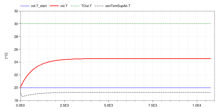
This completes the initial version of the model. When simulating the model, the response shown below should be seen.
If we were interested in computing electricity use for the pump, we could have used the same model as for the fan.
To explicitly model duct pressure drop, we could have added
Buildings.Fluid.FixedResistances.PressureDrop
to the model. However, computationally it is cheaper to lump these
pressure drops into other component models. In fact, rather than
separately computing the pressure drop of the heat recovery and the
air-side pressure drop of the cooling coil, we could have modeled
the cooling coil pressure drop as dp_nominal =
2*200+200 and set for the heat recovery dp1_nominal =
0 and dp2_nominal = 0. Setting the nominal
pressure drop to zero will remove this equation from the model.
| Name | Description |
|---|---|
| Medium for air | |
| Medium for water |
nominalValuesDefineDefaultPressureCurve=true
in the mover component to suppress a warning. This is for #3819.Modelica.Fluid.System to address issue
#311.