.Modelica_LinearSystems2.Controllers.Examples.SimpleControlledDrive

Information

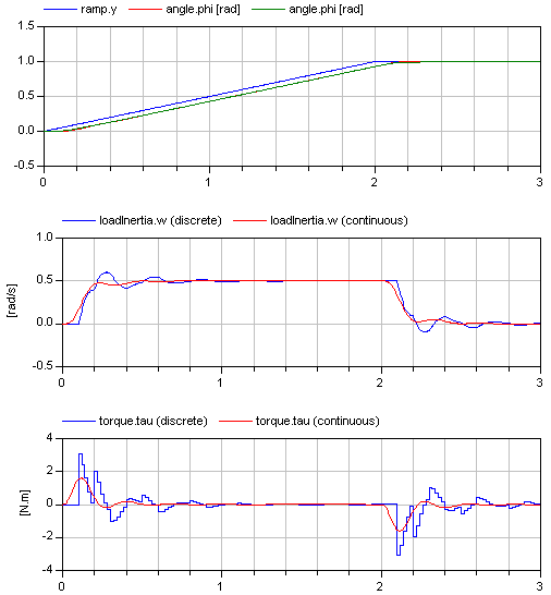
This example demonstrates the control of a simple model of a flexible drive system with a continuous or discrete P-PI cascade controller. Simulate for 3 s and plot

ramp.y          (reference angle of loadInertia)
loadInertia.phi (angle of loadInertia)
loadInertia.w   (speed of loadInertia)
torque.tau      (motor torque)

The standard setting in component sampleClock models a continuous controller. This means that all 3 samplers are just dummy components containing the equation "y=u" and that the PI component in the controller is a continuous PI controller.

Change sampleClock.blockType to "Discrete" block. By this global setting, the 3 sampler blocks and the PI speed controller are transformed into a discrete representation. The base sample time is defined in component sampleClock (= 0.02 s). Every discrete component samples its input and output. The sampling time of every component is a multiple of the base sample time (defined via parameter sampleFactor). Here, the sampler and the PI speed controller are sampled with the base sample frequency. The sample time of the 2 samplers and of the P position controller is a factor of 5 slower.

When comparing the simulations of the continuous and the (more realistic) discrete representation, it turns out that the discrete control systems works a bit worse. This can be improved by reducing the sample time in sampleClock.

The Controller library has several blocks to model this system even more realistically, e.g, by component AD converter to model the quantization errors of the analog measurement signals, component DA converter to model the quantization errors and computing time to determine the analog actuator (torque) signal, and component Noise to add uniformly distributed noise to the measurement signals.

Within Dymola simulation tool the "Commands / Simulate and Plot Results" selection plots the simulation result of either continuous or discrete controller.

Simulation results

In the following figure the simulation results of the discrete and of the continuous controller are compared.