At the top level of the Modelica_LinearSystems2 library, data structures are provided as Modelica records defining different representations of linear, time invariant differential and difference equation systems. In the record definitions, functions are provided that operate on the corresponding data structure. Currently, the following linear system representations are available:
| Representation | Description |
|---|---|
| record StateSpace | Multi input, multi output, linear differential equation systems
in state space form:
|
| record TransferFunction | Single input, single output, transfer functions defined via
a numerator and a denominator polynomial n(s) and d(s)
respectively:
|
| record ZerosAndPoles | Single input, single output, transfer function defined via the
products of its zeros z and poles p, respectively;
A description with zeros and poles is problematic: For
example, a small change in the imaginary part of
a conjugate complex pole pair, leads no longer to
a transfer function with real coefficients. If the same zero
or pole is present twice or more, then a diagonal state space
form is no longer possible. This means that the structure is very
sensitive if zeros or poles are close together. For this and other
reasons, internally, this data structure stores the zeros and poles
as first and second order polynomials with real coefficients:
|
| record DiscreteStateSpace | Multi input, multi output, linear difference equation system in
state space form:
withx(Ts*(k+1)) = A * x(Ts*k) + B * u(Ts*k) y(Ts*k) = C * x(Ts*k) + D * u(Ts*k) x_continuous(Ts*k) = x(Ts*k) + B2 * u(Ts*k) Ts the sample time and k the index
of the actual sample instance (k=0,1,2,3,...).
x(t) is the discrete state vector and
x_continuous(t) is the state vector of the
continuous system from which the discrete block has been derived by
a state transformation, in order to remove dependencies of
past values of u. |
It is planned to add linear system descriptions such as DiscreteFactorized, FrequencyResponse, and DiscreteFrequencyResponse, in the future. Furthermore, several useful functions are not yet available in the records above. They will also be added in the future.
Below, a typical session in the command window is shown:
import Modelica_LinearSystems2.TransferFunction
//  = true
import Modelica_LinearSystems2.ZerosAndPoles
//  = true

s = TransferFunction.s()
p = ZerosAndPoles.p()

tf1 = (s + 2)/(2*s^2 + 3*s +4)
String(tf1)
//  = "(s + 2)/(2*s^2 + 3*s + 4)"

zp1 = 4*(p + 1)/((p - 1)*(p^2 - 4*p + 13))
String(zp1)
//  = "4*(p + 1) / ( (p - 1)*(p^2 - 4*p + 13) )"

tf2 = ZerosAndPoles.Conversion.toTransferFunction(zp1)
tf2
// (4*s + 4)/(s^3 - 5*s^2 + 17*s - 13)

tf3 = tf1*tf2
tf3
// (4*s^2 + 12*s + 8)/(2*s^5 - 7*s^4 + 23*s^3 + 5*s^2 + 29*s - 52)

TransferFunction.Plot.bode(tf3)
The last command (Plot.bode) results in the
following frequency response:
Note, the frequency range of interest is automatically determined (it can be fairly well deduced from the phase information of poles and zeros).
Transfer function tf3 can be transformed into
a state space description with command ss =
StateSpace(tf3) and a poles-and-zeros plot and print
out is then available via
StateSpace.Plot.polesAndZeros(ss).
import Modelica_LinearSystems2.StateSpace
//  = true

ss = StateSpace(tf3)
StateSpace.Plot.polesAndZeros(ss)
resulting in:
It is also possible to linearize any Modelica model at the start
time (after initialization has been performed). This is especially
useful if the model is initialized in steady state. For example,
the command StateSpace.Import.fromModel("xxx") results
in:
ss2 = StateSpace.Import.fromModel("Modelica.Mechanics.Rotational.Examples.First")
ev = StateSpace.Analysis.eigenValues(ss2)
ev
// {-0.0595186 + 76.3757*j, -0.0595186 - 76.3757*j, -0.714296, 3.0963e-17}
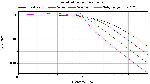
Also several filters are provided. Typical frequency responses of implemented filters are shown in the next figure:
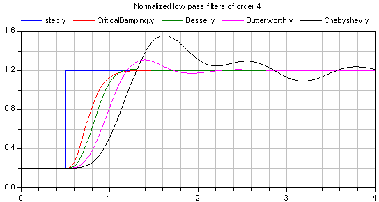
The step responses of the same low pass filters are shown in the next figure, starting from a steady state initial filter with initial input equal to 0.2: