.Modelica_LinearSystems2.UsersGuide.GettingStarted.Polynomials

Information

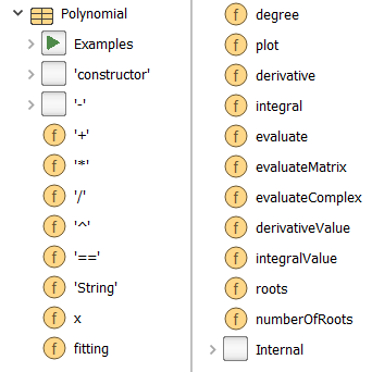
Polynomials with real coefficients are defined via record Modelica_LinearSystems2.Math.Polynomial. Read first the previous section about Complex numbers to understand how records, functions in records and the coming operator overloading technique works. The Polynomial record is equivalent to the Complex record. A screenshot is shown in the next figure:

A Polynomial is constructed by the command Polynomial(coefficientVector), where the input argument provides the polynomial coefficients in descending order. In the following figure, a typical session in the command window is shown (try it, e.g., in Dymola command window):

import Modelica_LinearSystems2.Math.Polynomial
// = true

x = Polynomial.x()
p1 = -6*x^2 + 4*x -3
p1
// -6*x^2 + 4*x - 3
String(p1)
//  = "-6*x^2 + 4*x - 3"

int_p = Polynomial.integral(p1)
String(int_p)
//  = "-2*x^3 + 2*x^2 - 3*x"

p2 = 3*p1
p3 = p2+p1
p3
// -24*x^2 + 16*x - 12

r = Polynomial.roots(p3, printRoots=true)
//  =
//    0.333333 + 0.62361*j
//    0.333333 - 0.62361*j

der_p = Polynomial.derivative(p1)
String(der_p)
//  = "-12*x + 4"

Polynomial.evaluate(der_p, 1)
//  = -8.0

After defining the import statement to get Polynomial as an abbreviation for Modelica_LinearSystems2.Math.Polynomial, the coefficients are given as vector input to Polynomial(). Via the operator-'String' function (called by String(p)) polynomial p is pretty printed. Besides all elementary operations, such as operator '+' or '*', functions to compute the integral or the derivative are provided. With function evaluate(..) the Polynomial is evaluated for a given value x. With function roots, the roots of the Polynomial are evaluated and are returned as a vector of complex numbers. If the optional second input argument printRoots is set to true, the roots are at once also nicely printed.

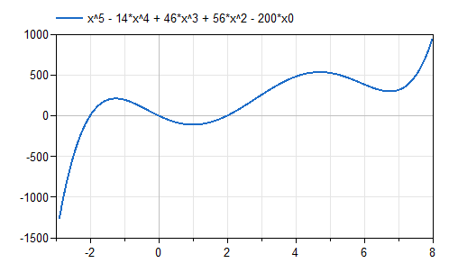
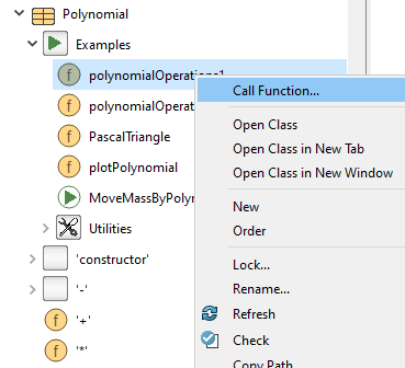
With function fitting(), a polynomial can be determined that approximates given table values. Finally with function plot(), the interesting range of x is automatically determined (via calculating the roots of the polynomial and of its derivative) and plotted. A typical plot is shown in the next figure:

Several other examples of Polynomial are available in Polynomial.Examples. In Dymola, select the function with the right mouse button and click "Ok" on the resulting menu which provides the possibility to define all the input arguments. Since the Examples function do not have any input arguments, only the "Ok" button is present: