packageChecksInFixedWindow_withFFT

Information

This library provides blocks that check properties based on FFT (Fast Fourier Transform) computations in fixed time windows. An FFT determines the frequency content and amplitudes of a sampled, periodic signal, and the blocks in this package check whether these frequencies and amplitudes fulfill certain conditions. The approach is to trigger the sampling of the periodic signal by a rising edge of Boolean input variable condition, storing the values in an internal buffer and computing the FFT once "sufficient" values are available.

Other blocks performing checks in a fixed time window are provided in sublibrary ChecksInFixedWindow.
Blocks performing checks in a sliding time window are provided in sublibrary ChecksInSlidingWindow.

All blocks of this library have the following interfaces:

• Real input u: The time signal on which the FFT computation is performed. This signal should be (at least approximately) periodic, after a rising edge of input condition.
• Boolean input condition: Whenever condition has a rising edge an FFT computation is triggered. This means that the input signal u is sampled and the sampled values are stored in an internal buffer. Once "enough" sample values are available, the FFT computation is performed.
  If the simulation ends before enough samples values are stored, then the remaining buffer of the FFT computation is filled with zeros ("zero-padding"), an FFT computation is performed and a warning message is printed. If condition has a rising edge before the buffer of the previous FFT computation was filled, the buffer of the previous FFT computation is reset and no FFT computation takes place. Instead, u is newly sampled and stored in the internal buffer.
  Whenever an FFT has been computed, the "check" of the respective block is evaluated. Note, condition is typically the output of a time locator from library TimeLocators.
• Property output y: If the check is successful, y = Property.Satisfied. If the check fails, y = Property.Violated. If neither of the two properties hold (for example before the first rising edge of input condition), y = Property.Undecided.
• Real output scaledDistance: The (scaled) "distance" between the FFT and its allowed domain.
  If y = Property.Undecided, scaledDistance = 1.
  If y = Property.Satisfied, scaledDistance ≥ 0.
  If y = Property.Violated, scaledDistance < 0.
  This signal can be used for example to formulate a constraint in an optimization setup.
• Boolean output FFT_computation: = true as long as input u is sampled and stored in an internal buffer. At the time instant where FFT_computation has a falling edge (changes from true to false), the FFT computation and afterwards the check is performed. Property output y gets a new value and keeps it until a new FFT computation is performed. This output can for example be used to stop the simulation once the FFT computation is finished. It also gives an indication how long the sampling of the input u is performed, until enough values are available to compute the FFT in the required precision.

All blocks of this library have the following features:

• The maximum frequency of interest f_max is either defined by a parameter, or is computed from other data. Internally, the FFT is computed with a frequency ≥ 10*f_max (more details see below).
• The frequency resolution f_resolution is a parameter that defines the resolution of the frequency axis. In particular all frequency points are an integer multiple of f_resolution. For example if f_resolution = 0.1, then the frequency axis of the FFT is {0, 0.1, 0.2, 0.3, ...}. It is highly recommended that f_resolution is selected in such a way that the frequencies of interest (such as a base frequency of 50 Hz) can be expressed as an integer multiple of f_resolution.
• The number of sample points of the FFT is not an input, but is computed as the smallest Integer number that fulfills the following conditions:
  • Maximum FFT frequency ≥ 10*f_max.
  • Frequency axis resolution is f_resolution.
  • The number of sample points can be expressed as 2^a*3^b*4^c*5^d (and a,b,c,d are appropriate Integers).
  • The number of sample points is even.
Note, in the original publication about the efficient computation of FFT (Cooley and Tukey, 1965), the number of sample points must be 2^a. However, all newer FFT algorithms do not have this strong restriction and especially not the open source software KissFFT from Mark Borgerding used in this package.

Before starting a simulation, the needed simulation time for the FFT is typically not known. You can handle this in the following way:

• If you just would like to determine an FFT of a signal, set the simulation time to a large value (say 100000 s) and terminate the simulation when output signal FFT_computed has a falling edge. You can use the block FallingEdgeTerminate for this purpose.
• Just use any simulation end time and inspect the result. If your simulation time is too short, a warning message is printed (in the warning message the minimum needed simulation time is displayed). If your simulation time is too long, inspect signal FFT_computed (a falling edge indicates when the FFT was computed).
• Use function realFFTinfo to determine the minimum simulation time and other characteristics of the desired FFT computation beforehand. For example calling this function as:

    realFFTinfo(f_max = 170, f_resolution = 0.3)

  results in the following output:

     ... Calculate FFT properties   
     Desired:
        f_max         = 170 Hz
        f_resolution  = 0.3 Hz
        f_max_factor  = 5
     Calculated:
        Number of sample points    = 5760 (= 2^7*3^2*5^1)
        Sampling frequency         = 1728 Hz (= 0.3*5760)
        Sampling period            = 0.000578704 s (= 1/1728)
        Maximum FFT frequency      = 864 Hz (= 0.3*5760/2; f={0,0.3,0.6,...,864} Hz)
        Number of frequency points = 2881 (= 5760/2+1)
        Simulation time            = 3.33275 s
  

In the icon of the blocks the last computed FFT is shown, see example in the next figure:

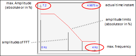
The Boolean parameter storeFFTonFile defines whether the result of every FFT computation is also stored on file (storeFFTonFile = true) or not. By default, every FFT computation is stored on a separate file in MATLAB 4 binary format. For example, if the FFT computation is performed in a model with the instance name "MyModel.Requirements.Rectifier.R2", then in the current directoy the following files will be stored (during initialization, all files FFT.* in directory MyModel are deleted in order to remove potentially old results. If directory MyModel does not exist, it is created):

   MyModel
     FFT.Requirements.Rectifier.R2.1.mat   // first FFT
     FFT.Requirements.Rectifier.R2.2.mat   // second FFT
       ...

All files consist of a matrix FFT[f,A] where the first column are the frequency values in [Hz] and the second column are the amplitudes at the corresponding frequency. The FFTs can be plotted with functions plot_FFT_fromFile, plot_FFTs_of_model, plot_FFTs_from_directory. For example, all FFTs of the last simulation run can be plotted by calling function plot_FFTs_of_model. The FFT plot of signal

     y = 5 + 3*sin(2*pi*2) + 1.5*sin(2*pi*3)

is shown in the next figure:

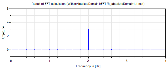
As can be seen, the mean value = 5 of y is present at f = 0 Hz. The amplitudes and frequencies of the two sin-functions are precisely reported in the plot. This FFT was computed with f_resolution = 0.2 Hz.

References

Mark Borgerding (2010):

KissFFT, version 1.3.0. http://sourceforge.net/projects/kissfft/.
 

James W. Cooley, John W. Tukey (1965):

An algorithm for the machine calculation of complex Fourier series. Math. Comput. 19: 297–301. doi:10.2307/2003354.
 

Martin R. Kuhn (2011):

Advanced generator design using pareto-optimization. 2011 IEEE Ninth International Conference on Power Electronics and Drive Systems (PEDS), pp. 1061 –1067, Dec. DOI: 10.1109/PEDS.2011.6147391.
 

Martin R. Kuhn, Martin Otter, Tim Giese (2015):

Model Based Specifications in Aircraft Systems Design. Modelica 2015 Conference, Versailles, France, pp. 491-500, Sept.23-25, 2015. Download from: http://www.ep.liu.se/ecp/118/053/ecp15118491.pdf

Contents

Name	Description
WithinAbsoluteDomain	A rising condition input triggers an FFT calculation. The amplitudes of the FFTs must be below a frequency dependent limit
WithinRelativeDomain	A rising condition input triggers an FFT calculation. The amplitudes of the FFTs must be below a frequency dependent limit that is defined relative to the amplitude of the base frequency
MaxTotalHarmonicDistortion	A rising condition input triggers an FFT calculation. The Total Harmonic Distortion (THD) of the FFTs must be below the given limit.
Internal	Library of internal components used by FFT blocks (should not be directly used)

Revisions