.OpenIPSL.Examples.Tutorial.Example_4.Instructions.AutomatingAnalysis

Information

Automating Analysis with Modelica functions

1. Open the diagram layer of the SMIBPartial model. Remember that this model is located in the following path: SMIB.BaseModels.BaseNetwork.
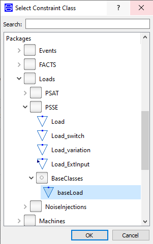
2. Double-click the load component and go to the Attributes tab. In the Properties group select the Replaceable option. Then click the Constraining clause checkbox and browse for class by pressing the button . From the package tree select OpenIPSL.Electrical.Loads.PSSE.BaseClasses.baseLoad as shown in the figure below.

   

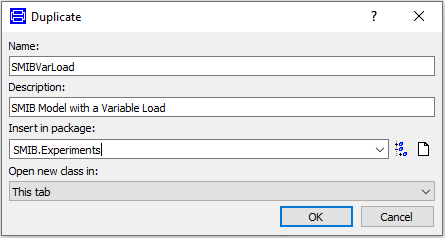
3. In the package browser, go to the Experiments package, create a new model by duplicating SMIB and name it SMIBVarLoad.

   

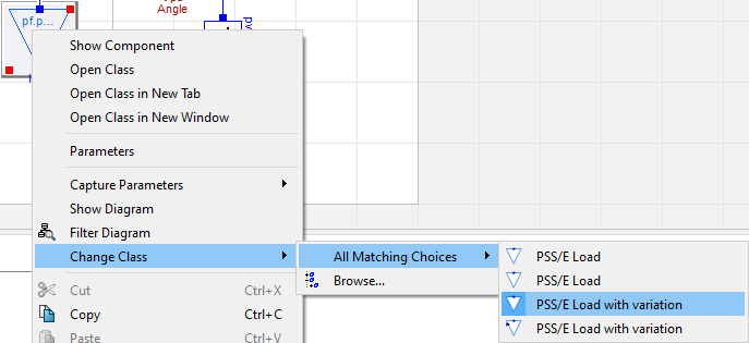
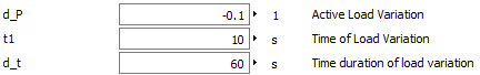
4. Now right-click the load component of the SMIBVarLoad model and change the class to PSS/E Load with variation as indicated in the following picture:

   

5. Double-click the load component to update its power flow parameters. You can either use the button to insert a component reference or type directly each value according to the following settings:

    

   • P_0: pf.powerflow.loads.PL1
   • Q_0: pf.powerflow.loads.QL1
   • v_0: pf.powerflow.bus.V3
   • angle_0: pf.powerflow.bus.A3

    

6. Specify a load drop of 0.1 pu starting at t = 10 sec and for a duration of 60 sec.

   

7. This time we want to see the effect of a perturbation on the load. Therefore, double-click the fault component and change its time parameters so that the fault event occurs after the new simulation stop time (100 sec).

   

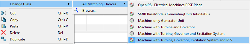
8. Change the class of the genunit component of the SMIBVarLoad model to the GeneratorTurbGovAVRPSS model. You will find it as "Machine with Turbine, Governor, Excitation System and PSS".

   

9. Go to the Simulation view and close all the results by right-clicking any of the results from the Variable Browser and then selecting the Close All Results option.

   

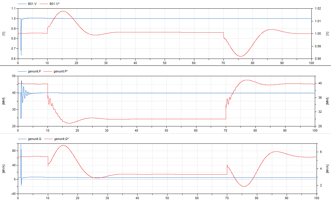
   We would like to automatically simulate the SMIB and SMIBVarLoad models and plot their results for comparative purposes. For this to be done we are going to create and call a Modelica function that includes the right sequence of steps.

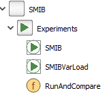
10. Create a new Modelica function inside of the Experiments package. For this to be done you can go to File > New > Function after selecting the package, or alternatively, you can right-click the package and then click on New > Function. Name the function RunAndCompare. The Experiments package should now look like this:

    

11. Go to the Modelica text of the RunAndCompare function and create 6 input variables as indicated below:

    function RunAndCompare
      "Runs different instances of the SMIB model to compare their results"
    
      // INPUTS TO THE FUNCTION
      input Modelica.Units.SI.Time tsim=100 "Simulation time";
      input Integer numberOfIntervalsin=10000 "No. of intervals";
      input String methodin = "Dassl" "Solver";
      input Real fixedstepsizein= 1e-3 "Time step - needed only for fixed time step solvers";
    
      // MODELS TO SIMULATE
      input String modelA="SMIB.Experiments.SMIB";
      input String modelB="SMIB.Experiments.SMIBVarLoad";
      ...
        

12. Add the following code inside of the algorithm section of the function to define the simulation and plotting instructions:

    algorithm 
      simulateModel(
        modelA,
        stopTime=tsim,
        numberOfIntervals=numberOfIntervalsin,
        method = methodin,
        fixedstepsize=fixedstepsizein,
        resultFile="res_casea");
      simulateModel(
        modelB,
        stopTime=tsim,
        numberOfIntervals=numberOfIntervalsin,
        method = methodin,
        fixedstepsize=fixedstepsizein,
        resultFile="res_caseb");
    
      removePlots(true);
      Advanced.FilesToKeep :=10;
      createPlot(id=1, position={15, 15, 678, 703}, y={"B01.V"},
        range={0.0, 10.0, 0.4, 1.4}, grid=true, filename="res_casea.mat",
        colors={{28,108,200}}, displayUnits={"1"});
      createPlot(id=1, position={15, 15, 678, 703}, y={"genunit.P"},
        range={0.0, 10.0, -1.5, 2.0}, grid=true, subPlot=102,
        colors={{28,108,200}}, displayUnits={"1"});
      createPlot(id=1, position={15, 15, 678, 703}, y={"genunit.Q"},
        range={0.0, 10.0, -0.5, 2.0}, grid=true, subPlot=103,
        colors={{28,108,200}}, displayUnits={"1"});
      createPlot(id=1, position={15, 15, 678, 703}, y={"B01.V"},
        range={0.0, 10.0, 0.4, 1.4}, erase=false, grid=true,
        filename="res_caseb.mat", colors={{238,46,47}}, displayUnits={"1"},
        axes={2});
      createPlot(id=1, position={15, 15, 678, 703}, y={"genunit.P"},
        range={0.0, 10.0, -1.5, 2.0}, erase=false, grid=true, subPlot=102,
        colors={{238,46,47}}, displayUnits={"1"},
        axes={2});
      createPlot(id=1, position={15, 15, 678, 703}, y={"genunit.Q"},
        range={0.0, 10.0, -0.5, 2.0}, erase=false, grid=true, subPlot=103,
        colors={{238,46,47}}, displayUnits={"1"},
        axes={2});
    
    end RunAndCompare;
      

13. Right-click the RunAndCompare function, select the Call Function... option and then press OK. If everything goes well you will get the plots shown below.