.OpenIPSL.Examples.Tutorial.Example_4.Instructions.PopulatingRecords

Populating PF Records

Information

Populating Power Flows with GridCal

The next step is to populate our model with power flow results generated from GridCal. For simplicity, we will create a power flow model from an accompanying PSS/E .raw. However, it is possible to run the power flows from a native GridCal model.

Create a new PSSE_Files folder within SMIB_Example/models/SMIB folder.

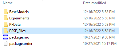
Create a new PSS/E raw file called SMIB_Base_Case.raw within the PSSE_Files folder. Copy and paste the following text inside the file and save it:

0,   100.00, 33, 0, 1, 50.00     / PSS(R)E-33.4    FRI, FEB 26 2021  16:31
SMIB

     1,'B01         ', 100.0000,2,   1,   1,   1,1.00000,   4.0463,1.10000,0.90000,1.10000,0.90000
     2,'B02         ', 100.0000,3,   1,   1,   1,1.00000,   0.0000,1.10000,0.90000,1.10000,0.90000
     3,'B03         ', 100.0000,1,   1,   1,   1,0.99598,  -0.2870,1.10000,0.90000,1.10000,0.90000
     4,'B04         ', 100.0000,1,   1,   1,   1,0.99199,  -0.5763,1.10000,0.90000,1.10000,0.90000
0 / END OF BUS DATA, BEGIN LOAD DATA
     4,'1 ',1,   1,   1,    50.000,    10.000,     0.000,     0.000,     0.000,     0.000,   1,1,0
0 / END OF LOAD DATA, BEGIN FIXED SHUNT DATA
0 / END OF FIXED SHUNT DATA, BEGIN GENERATOR DATA
     1,'1 ',    40.000,     5.417,    60.000,     0.000,1.00000,     0,   100.000, 0.00000E+0, 2.00000E-1, 0.00000E+0, 0.00000E+0,1.00000,1,  100.0,    80.000,     0.000,   1,1.0000
     2,'1 ',    10.017,     8.007,    60.000,     0.000,1.00000,     0,   100.000, 0.00000E+0, 2.00000E-1, 0.00000E+0, 0.00000E+0,1.00000,1,  100.0,    80.000,     0.000,   1,1.0000
0 / END OF GENERATOR DATA, BEGIN BRANCH DATA
     1,     4,'1 ', 1.00000E-3, 2.00000E-1,   0.00000,    0.00,    0.00,    0.00,  0.00000,  0.00000,  0.00000,  0.00000,1,1,   0.00,   1,1.0000
     2,     3,'1 ', 5.00000E-4, 1.00000E-1,   0.00000,    0.00,    0.00,    0.00,  0.00000,  0.00000,  0.00000,  0.00000,1,2,   0.00,   1,1.0000
     2,     4,'1 ', 1.00000E-3, 2.00000E-1,   0.00000,    0.00,    0.00,    0.00,  0.00000,  0.00000,  0.00000,  0.00000,1,2,   0.00,   1,1.0000
     3,     4,'1 ', 5.00000E-4, 1.00000E-1,   0.00000,    0.00,    0.00,    0.00,  0.00000,  0.00000,  0.00000,  0.00000,1,2,   0.00,   1,1.0000
0 / END OF BRANCH DATA, BEGIN TRANSFORMER DATA
0 / END OF TRANSFORMER DATA, BEGIN AREA DATA
0 / END OF AREA DATA, BEGIN TWO-TERMINAL DC DATA
0 / END OF TWO-TERMINAL DC DATA, BEGIN VSC DC LINE DATA
0 / END OF VSC DC LINE DATA, BEGIN IMPEDANCE CORRECTION DATA
0 / END OF IMPEDANCE CORRECTION DATA, BEGIN MULTI-TERMINAL DC DATA
0 / END OF MULTI-TERMINAL DC DATA, BEGIN MULTI-SECTION LINE DATA
0 / END OF MULTI-SECTION LINE DATA, BEGIN ZONE DATA
0 / END OF ZONE DATA, BEGIN INTER-AREA TRANSFER DATA
0 / END OF INTER-AREA TRANSFER DATA, BEGIN OWNER DATA
0 / END OF OWNER DATA, BEGIN FACTS DEVICE DATA
0 / END OF FACTS DEVICE DATA, BEGIN SWITCHED SHUNT DATA
0 / END OF SWITCHED SHUNT DATA, BEGIN GNE DATA
0 / END OF GNE DATA, BEGIN INDUCTION MACHINE DATA
0 / END OF INDUCTION MACHINE DATA
Q

Execute run_pf.py from a terminal.

python run_pf.py SMIB

(openipsl_tutorial) c:\Users\Miguel\SMIB_Example>python run_pf.py SMIB
It 0, error 0.5, converged False, x [0. 0. 0. 1. 1.], dx not computed yet
--------------------------------------------------------------------------------------------------------------------------------------------------------------------------------------------------------
Iter: 1
--------------------------------------------------------------------------------------------------------------------------------------------------------------------------------------------------------
It 1, error 0.016918884074426793, converged False, x [ 0.07000175 -0.00498304 -0.00996608  0.99658333  0.99316667], dx [ 0.07000175 -0.00498304 -0.00996608 -0.00341667 -0.00683333]
--------------------------------------------------------------------------------------------------------------------------------------------------------------------------------------------------------
Iter: 2
--------------------------------------------------------------------------------------------------------------------------------------------------------------------------------------------------------
It 2, error 2.1358057256101737e-05, converged False, x [ 0.07061997 -0.00500866 -0.01005764  0.99598493  0.99199502], dx [ 0.00061822 -0.00002562 -0.00009156 -0.00059841 -0.00117164]
--------------------------------------------------------------------------------------------------------------------------------------------------------------------------------------------------------
Iter: 3
--------------------------------------------------------------------------------------------------------------------------------------------------------------------------------------------------------
It 3, error 3.453681785003937e-11, converged False, x [ 0.0706208  -0.00500868 -0.01005778  0.99598418  0.99199354], dx [ 0.00000083 -0.00000002 -0.00000014 -0.00000075 -0.00000148]
--------------------------------------------------------------------------------------------------------------------------------------------------------------------------------------------------------
Iter: 4
--------------------------------------------------------------------------------------------------------------------------------------------------------------------------------------------------------
It 4, error 3.802513859341161e-15, converged True, x [ 0.0706208  -0.00500868 -0.01005778  0.99598418  0.99199354], dx [ 0. -0. -0. -0. -0.]

(openipsl_tutorial) c:\Users\Miguel\SMIB_Example>

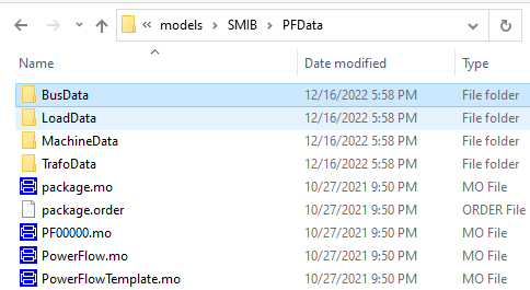
📌 A new power flow record called PF00000 should be generated inside the PFData subfolder.

Refresh your model. You should get a new file called PF0000.mo inside your PFData folder. In fact, there should be a new file in every subfolder too.
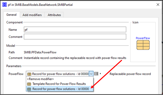
In the diagram layer of your SMIB model, double click the power flow component pf. Select the newly created power flow PF00000 as the value for the PowerFlow field. By doing so, we are specifying that the model will initialize using the power flow results in that specific container.
📌 You can alternatively modify the Modelica Text of the SMIB Experiment model as follows:
```
model SMIB
  extends Modelica.Icons.Example;
  extends BaseModels.BaseNetwork.SMIBPartial(pf(redeclare record PowerFlow = PFData.PF00000));
  replaceable BaseModels.GeneratingUnits.GeneratorOnly       genunit...
equation
  ...
  annotation ...
end SMIB;
    
```
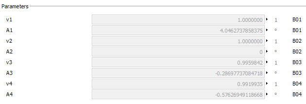
To see the power flow values in Dymola, click on the square button on the left of the PowerFlow selection menu.

You should see that the power flow record is composed of four fields: bus, load, machine and transformer.

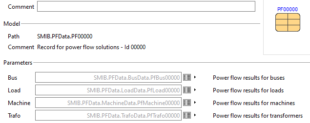
Inside each field, we can detail the power flow results
Simulate the SMIB model for 2 seconds. Plot the voltage buses. Notice that the power flow solution initializes the dynamical simulation in an equilibrium (i.e., flat) so that the states of the system are not changing.

Generated at 2026-03-12T19:14:05Z by OpenModelicaOpenModelica 1.26.3 using GenerateDoc.mos