
packageUsersGuide
Extends from Modelica.Icons.Information (Icon for general information packages).
Information
This package contains models for fans and pumps (movers). The same models can be used for fans or pumps.
Model description
The models consider the pressure rise, flow rate, speed, power consumption, and heat dissipation based on the user's specification. They can take pressure rise (head), mass flow rate, or speed (absolute or relative) as control signal, and compute resulting quantities based on user-provided performance curves.
While the models in the package Buildings.Fluid.Movers allow full customization, preconfigured models that use the same underlying physical equations are available in the package Buildings.Fluid.Movers.Preconfigured. The models in Buildings.Fluid.Movers can also be parameterized with the data records from Buildings.Fluid.Movers.Data.
A detailed description of the fan and pump models can be found in Wetter (2013). The models are implemented as described in this paper, except that equation (20) is no longer used. The reason is that the transition (24) caused the derivative
d Δp(r(t), V(t)) ⁄ d r(t)
to have an inflection point in the regularization region r(t) ∈ (δ/2, δ). This caused some models to not converge. To correct this, for r(t) < δ, the term V(t) ⁄ r(t) in (16) has been modified so that (16) can be used for any value of r(t).
Below, the models are briefly described.
Performance data
The models use performance curves that compute pressure rise, electrical power draw and efficiency as a function of the volume flow rate and the speed. The following performance curves are implemented:
| Independent variable | Dependent variable | Record for performance data | Function |
|---|---|---|---|
| Volume flow rate | Pressure | flowParameters | pressure |
| Volume flow rate | Efficiency (hydraulic or motor) |
efficiencyParameters | efficiency |
| Motor part load ratio | Motor efficiency* | efficiencyParameters_yMot | efficiency_yMot |
| Volume flow rate | Power** | powerParameters | power |
Notes (applicable to Buildings.Fluid.Movers.FlowControlled_dp and Buildings.Fluid.Movers.FlowControlled_m_flow):
- * The models will ignore this record if the nominal motor power is not provided and cannot be estimated from the pressure curve. This is because calculating the motor part load ratio requires knowing the nominal power.
- ** The models will ignore this record if the pressure curve is not provided and the speed is unknown. This is because the models wouldn't be able to compute the elctrical power correctly using similarity laws without speed. In this case the user should consider using the preconfigured mover models in Buildings.Fluid.Movers.Preconfigured which will auto-populate a pressure curve from nominal flow rate and pressure.
These performance curves are implemented in Buildings.Fluid.Movers.BaseClasses.Characteristics, and are used in the performance records in the package Buildings.Fluid.Movers.Data. The package Buildings.Fluid.Movers.Data contains different data records.
Models that use performance curves for pressure rise
The model Buildings.Fluid.Movers.SpeedControlled_y takes as an input a control signal between 0 and 1. From this input and the current flow rate, they compute the pressure rise. This pressure rise is computed using a user-provided list of operating points that defines the fan or pump curve at full speed. For other speeds, similarity laws are used to scale the performance curves, as described in Buildings.Fluid.Movers.BaseClasses.Characteristics.pressure.
For example, suppose a pump needs to be modeled whose pressure versus flow relation crosses, at full speed, the points shown in the table below.
| Volume flow rate [m3⁄s] | Head [Pa] |
|---|---|
| 0.0003 | 45000 |
| 0.0006 | 35000 |
| 0.0008 | 15000 |
Then, a declaration would be
  Buildings.Fluid.Movers.SpeedControlled_y pum(
    redeclare package Medium = Medium,
    per.pressure(V_flow={0.0003,0.0006,0.0008},
                 dp    ={45,35,15}*1000))
    "Circulation pump";
This will model the following pump curve for the pump input signal y=1.
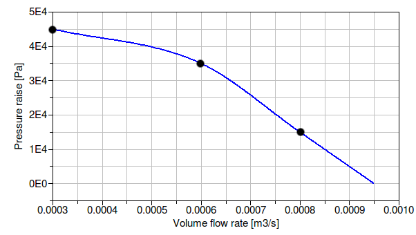
See Buildings.Fluid.Movers.Validation.PressureCurve for a small example that validates the pressure curve specification.
Models that directly control the head or the mass flow rate
The models Buildings.Fluid.Movers.FlowControlled_dp and Buildings.Fluid.Movers.FlowControlled_m_flow take as an input the pressure difference or the mass flow rate. This pressure difference or mass flow rate will be provided by the fan or pump, i.e., the fan or pump has idealized perfect control and infinite capacity. Using these models that take as an input the head or the mass flow rate often leads to smaller system of equations compared to using the models that take as an input the speed. The validation model Buildings.Fluid.Movers.Validation.ComparePowerInput demonstrates that the models with different input signals produce the same power consumption estimates.
These models can be configured for three different control inputs. For Buildings.Fluid.Movers.FlowControlled_dp, the head is as follows:
-
If the parameter
inputType==Buildings.Fluid.Types.InputType.Continuous, the head isdp=dp_in, wheredp_inis an input connector. -
If the parameter
inputType==Buildings.Fluid.Types.InputType.Constant, the head isdp=constantHead, whereconstantHeadis a parameter. -
If the parameter
inputType==Buildings.Fluid.Types.InputType.Stages, the head isdp=heads, whereheadsis a vectorized parameter. For example, if a mover has two stages and the head of the first stage should be 60% of the nominal head and the second stage equal todp_nominal, setheads={0.6, 1}*dp_nominal. Then, the mover will have the following heads:input signal stageHead [Pa] 0 0 1 0.6*dp_nominal 2 dp_nominal
Similarly, for Buildings.Fluid.Movers.FlowControlled_m_flow, the mass flow rate is as follows:
-
If the parameter
inputType==Buildings.Fluid.Types.InputType.Continuous, the mass flow rate ism_flow=m_flow_in, wherem_flow_inis an input connector. -
If the parameter
inputType==Buildings.Fluid.Types.InputType.Constant, the mass flow rate ism_flow=constantMassFlowRate, whereconstantMassFlowRateis a parameter. -
If the parameter
inputType==Buildings.Fluid.Types.InputType.Stages, the mass flow rate ism_flow=massFlowRates, wheremassFlowRatesis a vectorized parameter. For example, if a mover has two stages and the mass flow rate of the first stage should be 60% of the nominal mass flow rate and the second stage equal tom_flow_nominal, setmassFlowRates={0.6, 1}*m_flow_nominal. Then, the mover will have the following mass flow rates:input signal stageMass flow rates [kg/s] 0 0 1 0.6*m_flow_nominal 2 m_flow_nominal
These two models do not need to use a performance curve for the flow characteristics. The reason is that
- for given pressure rise (or mass flow rate), the mass flow rate (or pressure rise) is computed from the flow resistance of the duct or piping network, and
- at zero pressure difference, solving for the flow rate and the revolution leads to a singularity.
However, the computation of the electrical power consumption requires the mover speed to be known and the computation of the mover speed requires the performance curves for the flow and efficiency/power characteristics. Therefore these performance curves do need to be provided if the user desires a correct electrical power computation. If the curves are not provided, a simplified computation is used, where the efficiency curve is used and assumed to be correct for all speeds. This loss of accuracy has the advantage that it allows to use the mover models without requiring flow and efficiency/power characteristics.
The model
Buildings.Fluid.Movers.FlowControlled_dp
has an option to control the mover such
that the pressure difference set point is obtained
across two remote points in the system.
To use this functionality
parameter prescribeSystemPressure has
to be enabled and a differential pressure measurement
must be connected to
the pump input dpMea.
This functionality is demonstrated in
Buildings.Fluid.Movers.Validation.FlowControlled_dpSystem.
The models
Buildings.Fluid.Movers.FlowControlled_dp and
Buildings.Fluid.Movers.FlowControlled_m_flow
both have a parameter m_flow_nominal. For
Buildings.Fluid.Movers.FlowControlled_m_flow, this parameter
is used for convenience to set a default value for the parameters
constantMassFlowRate and
massFlowRates.
For both models, the value is also used for the following:
- To compute the size of the fluid volume that can be used to approximate the inertia of the mover if the energy dynamics is selected to be dynamic.
-
To compute a default pressure curve if no pressure curve has been specified
in the record
per.pressure. The default pressure curve is the line that intersects(dp, V_flow) = (dp_nominal, 0)and(dp, V_flow) = (m_flow_nominal/rho_default, 0). - To regularize the equations near zero flow rate to ensure a numerically robust model.
However, otherwise m_flow_nominal does not affect the mass flow rate of the mover as
the mass flow rate is determined by the input signal or the above explained parameters.
Electrical power consumption
All models compute the motor power draw Pele, the hydraulic power input Ẇhyd, the flow work Ẇflo and the heat dissipated into the medium Q̇. Based on the first law, the flow work is
Ẇflo = | V̇ Δp |,
where V̇ is the volume flow rate and Δp is the pressure rise. In order to prevent the model from producing negative mover power when either the flow rate or pressure rise is forced to be negative, the flow work Ẇflo is constrained to be non-negative. The regularisation starts around 0.01% of the characteristic maximum power Ẇmax = V̇max Δpmax. See discussions and an example of this situation in IBPSA, #1621.
The heat dissipated into the medium is as follows:
If the motor is cooled by the fluid, as indicated by
per.motorCooledByFluid=true, then the heat dissipated into the medium is
Q̇ = Pele - Ẇflo.
If per.motorCooledByFluid=false, then the motor is outside the fluid stream,
and only the shaft, or hydraulic, work Ẇhyd enters the thermodynamic
control volume. Hence,
Q̇ = Ẇhyd - Ẇflo.
The efficiencies are defined as
η = Ẇflo ⁄ Pele = ηhyd ηmot
ηhyd = Ẇflo ⁄ Ẇhyd
ηmot = Ẇhyd ⁄ Pele
where η is the total efficiency, ηhyd is the hydraulic efficiency, and ηmot is the motor efficiency. From the definition one has
η = ηhyd ηmot.
Hydraulic efficiency
The following options are used to specify how ηhyd is computed.
-
Efficiency_VolumeFlowRate- The user provides an array of ηhyd vs. V̇. If the array has only one element, ηhyd is considered constant. If the array has more than one element, the efficiency is interpolated or extrapolated using Buildings.Fluid.Movers.BaseClasses.Characteristics.efficiency. -
Power_VolumeFlowRate- The user provides an array of Ẇhyd vs. V̇. The power is interpolated or extrapolated using Buildings.Fluid.Movers.BaseClasses.Characteristics.power. ηhyd is then computed from Ẇhyd. -
EulerNumber(default 1) - The model uses a triple (ηhyd, V̇, Δp) corresponding to the operating point at which the peak efficiency is attained. It computes ηhyd and Ẇhyd using the package Buildings.Fluid.Movers.BaseClasses.Euler. The model finds ηhyd by evaluating the following correlation:
where x=log10(Eu ⁄ Eup), with the subscript p denoting the condition where the mover is operating at peak efficiency. The Euler number is defined as
Eu=(pressure forces)/(inertial forces)
from which one can derive the ratio of Euler numbers as
Eu ⁄ Eup =(Δp ⁄ V̇2) ⁄ (Δpp ⁄ V̇p2).
The peak point can be provided directly by the user or computed by calling the function Buildings.Fluid.Movers.BaseClasses.Euler.getPeak. This function finds the peak point when both pressure and power curves are provided. When only the pressure curve is available, the function estimates the peak point to be at V̇=V̇max ⁄ 2. Examples:
- Buildings.Fluid.Movers.Examples.StaticReset specifies the peak point directly.
- Buildings.Fluid.Movers.BaseClasses.Validation.EulerComparison implicitly calls the function when Buildings.Fluid.Movers.Data.Generic is instantiated.
For simplicity, the implementation does not directly use this method to estimate ηhyd at any operation point. Rather, it only computes a power curve at nominal speed and then uses similarity laws to estimate power at reduced speeds. Because the Euler number method does not account for the efficiency degradation along any curve Δp=kV̇2, these two methods are equivalent. See the documentation of Buildings.Fluid.Movers.BaseClasses.Euler.power for more details. Also see Buildings.Fluid.Movers.BaseClasses.Validation.EulerReducedSpeed for demonstration.
For more information on the Euler number method, see the documentation of Buildings.Fluid.Movers.BaseClasses.Euler.correlation, EnergyPlus 9.6.0 Engineering Reference chapter 16.4 equations 16.209 through 16.218, and Fu et al. (2022)
-
NotProvided(default 2) - The information of this efficiency item is not provided. The model uses a constant value ηhyd=0.7.
These options are validated in Buildings.Fluid.Movers.BaseClasses.Validation.HydraulicEfficiencyMethods and Buildings.Fluid.Movers.Validation.ComparePowerHydraulic.
The model uses EulerNumber as the default option
unless a pressure curve is not provided.
In this case, the model overrides it and uses NotProvided instead.
The user can use the same options to specify the total efficiency η
instead by setting per.powerOrEfficiencyIsHydraulic=false.
This changes the default constant value to η=0.49 and also imposes
an additional constraint of ηhyd ≤ 1 to prevent the division
ηhyd = η ⁄ ηmot
from producing efficiency values larger than one.
This configuration is validated in
Buildings.Fluid.Movers.BaseClasses.Validation.TotalEfficiencyMethods and
Buildings.Fluid.Movers.Validation.ComparePowerTotal.
Although the Euler number method is defined for ηhyd, this implementation applies it also to η and Pele as an approximation. The basis is that ηmot is mostly constant for motors larger than about 3.5 kW or 5 HP except when the motor part load drops below around 40%, (see the documentation of Buildings.Fluid.Movers.BaseClasses.Characteristics.motorEfficiencyCurve) which shows that η and ηhyd are roughly linear to each other for motors of this size.
Motor efficiency
The following options are used to specify how ηmot is computed.
-
Efficiency_VolumeFlowRate- This is same as the option for ηhyd with the same name. -
Efficiency_MotorPartLoadRatio- The user provides an array of ηmot vs. motor part load ratio ymot=Whyd ⁄ Pmot,nominal. The efficiency is interpolated or extrapolated using Buildings.Fluid.Movers.BaseClasses.Characteristics.efficiency_yMot. See Buildings.Fluid.Movers.BaseClasses.Validation.MotorEfficiencyMethods as an example. -
GenericCurve(default 1) - The user provides the rated motor power Pmot,nominal and maximum motor efficiency ηmot,max. The model then uses a generic motor efficiency curve as a function of motor PLR generated using Buildings.Fluid.Movers.BaseClasses.Characteristics.motorEfficiencyCurve. The ηmot,max is assumed to be 0.7 if not specified by user. If Pmot,nominal is unspecified, the model estimates it in the following ways:-
If a power curve is provided,
-
If the curve refers to total electric power Pele,
Pmot,nominal= Ẇmax,
where Ẇmax is the maximum value on the provided power curve. -
If the curve refers to hydraulic power Ẇhyd,
Pmot,nominal= 1.2 Ẇmax,
where the factor 1.2 accounts for a 20% oversize of the motor.
-
If the curve refers to total electric power Pele,
-
Otherwise, if only a pressure curve is provided,
Pmot,nominal= 1.2 (V̇max ⁄ 2) (Δpmax ⁄ 2) ⁄ ηhyd,p,
where the factor 1.2 also assumes a 20% oversize and the assumed peak hydraulic efficiency ηhyd,p=0.7 unless a hydraulic peak value is available in the record.
Efficiency_MotorPartLoadRatio. -
If a power curve is provided,
-
NotProvided(default 2) - The information of this efficiency item is not provided. The model uses a constant value ηmot=0.7.
These options are tested in Buildings.Fluid.Movers.BaseClasses.Validation.MotorEfficiencyMethods.
By default, the model uses the GenericCurve to obtain more accurate
results with variable ηmot. There are two exceptions:
-
When neither pressure curve nor nominal motor power is provided,
the model overrides it and uses
NotProvidedinstead. -
When the user specifies that the provided power is total power instead of
hydraulic power, i.e.
per.powerOrEfficiencyIsHydraulic==false, the model usesNotProvidedas default. The user can still mannually set it toGenericCurve, but this is not recommended. There are two reasons:-
Consider the following two equations:
ηmot = f(Ẇhyd),
where f(⋅) refers to the curve of motor efficiency vs. motor PLR. When Ẇhyd is known (i.e.
Pele = Ẇhyd ⁄ ηmot,per.powerOrEfficiencyIsHydraulic=true), the unknowns are ηmot and Pele which can be solved explicitly. Otherwise, the unknowns are ηmot and Ẇhyd, and an iterative solution would be required which may not converge for some values. - If the power data provided refer to the total electric power instead of the hydraulic power of the mover, it is likely that the mover comes with built-in motors. This is often the case for small pumps whose motor is inside the fluid stream (such as the pumps whose data are provided in Buildings.Fluid.Movers.Data.Pumps.Wilo). Because the models only use the two efficiencies to differentiate mover heat carried away by the fluid and dissipated to the ambient and now only a negligible amount of heat dissipates into the ambient, the separation of ηhyd and ηmot is then not important.
-
Consider the following two equations:
Start-up and shut-down transients
All models have a parameter use_riseTime. This
parameter affects the fan output as follows:
-
If
use_riseTime=false, then the input signaly(orm_flow_in, ordp_in) is equal to the fan speed (or the mass flow rate or pressure rise). Thus, a step change in the input signal causes a step change in the fan speed (or mass flow rate or pressure rise). -
If
use_riseTime=true, which is the default, then the fan speed (or the mass flow rate or the pressure rise) changes linear in time until it reaches the control input. The parameterriseTime, which by default is set to 30 seconds, determines how fast the speed changes. For example, ifriseTime=30seconds and the current speed is 0, then a step change in the fan input signal from 0 to 1 will cause the fan speed to increase its speed linearly to the full speed within 30 seconds. Similarly, if the fan speed is then reduced by changing the input signal from 1 to 0.5, it will take 15 seconds to achieve the new set point.
The figure below shows for a fan with use_riseTime=true
and riseTime=30 seconds the
speed input signal and the actual speed.

Although many simulations do not require such a detailed model
that approximates the transients of fans or pumps, it turns
out that using such a continuous change in speed can reduce computing time and
can lead to fewer convergence problems in large system models, because
a sudden change in control signal, such as when
a fan switches on, is damped before it affects the air flow rate.
This continuous change in flow rate turns out to be easier, and in
some cases faster, to simulate compared to a step change.
For most simulations, we therefore recommend to use the default settings
of use_riseTime=true and riseTime=30 seconds.
An exception are situations in which the fan or pump is operated at a fixed speed during
the whole simulation. In this case, set use_riseTime=false.
Note that if the fan is part of a closed loop control, then the value of riseTime affects
the transient response of the control.
When changing the value of riseTime, the control gains
may need to be retuned.
We now present values control parameters that seem to work in most cases.
Suppose there is a closed loop control with a PI-controller
Buildings.Controls.Continuous.LimPID
and a fan or pump, configured with use_riseTime=true and riseTime=30 seconds.
Assume that the transient response of the other dynamic elements in the control loop is fast
compared to the value of riseTime.
Then, a proportional gain of k=0.5 and an integrator time constant of
Ti=15 seconds often yields satisfactory closed loop control performance.
These values may need to be changed for different applications as they are also a function
of the loop gain.
If the control loop shows oscillatory behavior, then reduce k and/or increase Ti.
If the control loop reacts too slow, do the opposite.
Fluid volume of the component
All models can be configured to have a fluid volume at the low-pressure side. Adding such a volume sometimes helps the solver to find a solution during initialization and time integration of large models.
Enthalpy change of the component
If per.motorCooledByFluid=true, then
the enthalpy change between the inlet and outlet fluid port is equal
to the electrical power Pele that is consumed by the component.
Otherwise, it is equal to the hydraulic work Whyd.
The parameter addPowerToMedium, which is by default set to
true, can be used to simplify the equations.
If addPowerToMedium = false, then no enthalpy change occurs between
inlet and outlet.
This can lead to simpler equations, but the temperature rise across the component
will be zero. In particular for fans, this simplification may not be permissible.
Differences to models in Modelica.Fluid.Machines
The models in this package differ from Modelica.Fluid.Machines primarily in the following points:
-
They use a different base class, which allows to have zero mass flow rate.
The models in
Modelica.Fluidrestrict the number of revolutions, and hence the flow rate, to be non-zero. -
For the model with prescribed pressure, the input signal is the
pressure difference between the two ports, and not the absolute
pressure at
port_b. -
The pressure calculations are based on total pressure in Pascals instead of the pump head in meters.
This change was done to avoid ambiguities in the parameterization if the models are used as a fan
with air as the medium. The original formulation in
Modelica.Fluid.Machines converts head
to pressure using the density
medium.d. Therefore, for fans, head would be converted to pressure using the density of air. However, for pumps, manufacturers typically publish the head in millimeters water (mmH2O). Therefore, to avoid confusion when using these models with media other than water, we changed the models to use total pressure in Pascals instead of head in meters. - The performance data are interpolated using cubic hermite splines instead of polynomials. These functions are implemented in Buildings.Fluid.Movers.BaseClasses.Characteristics.
- The efficiency calculation is different, in particular, the models in this package allow use of the Euler number to compute the hydraulic efficiency.
References
Michael Wetter. Fan and pump model that has a unique solution for any pressure boundary condition and control signal. Proc. of the 13th Conference of the International Building Performance Simulation Association, p. 3505-3512. Chambery, France. August 2013.
Hongxiang Fu, David Blum, Michael Wetter. Fan and Pump Efficiency in Modelica based on the Euler Number. Proc. of the American Modelica Conference 2022, p. 19-25. Dallas, TX, USA. October 2022. https://doi.org/10.3384/ECP2118619